Practical 4: Pump Performance

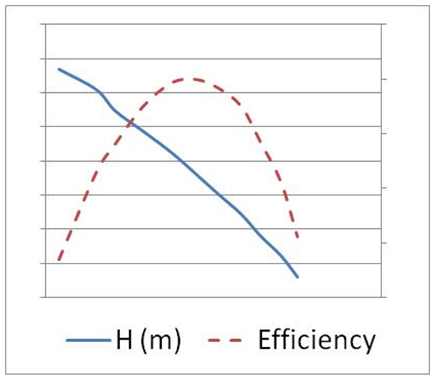
 Calculations

Part 1. Design Point

As we were not given a “design point” for this pump, you will need to determine (as accurately as possible) the H/Q combination corresponding to maximum efficiency – we will assume that this is the design point for this pump.

You can determine the efficiency of the pump (assuming constant P_elec = 80 watts) for each H-Q combination given in the manufacturer’s pump data, and produce a plot of head and efficiency versus discharge (hint: plot “head” on the primary axis and efficiency on the “secondary axis”). Include these calculations and the graph, plus the resultant design point, in your report.

Part 2. Operating Point

You need to determine a unique system curve for each pipe system tested (note that a “pipe system” is each unique combination of diameter, length and static lift – so there were 24 such systems altogether). This is most easily done in a spreadsheet program where you can set up the formulas and then simply change the parameters to determine a new system curve.

Supporting Information

Pump Data

The following data is from the pump manufacturer

(Note: LPH = litres per hour)

 Q (LPH) Height (m)

300             3.35

1100            3.05

1500            2.75

2100            2.44

2700            2.13

3200            1.83

3700            1.52

4200            1.22

4600             0.91

5050             0.61

5400            0.30

Power consumption = 80 watts (we assume this is relatively constant, irrespective of H and Q).

Assemble the given pump performance data to plot the H-Q performance curve.

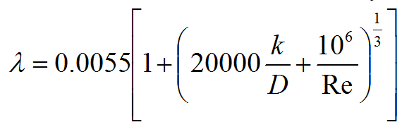
Calculation steps

For each combination of pipe diameter, pipe length and static lift, you must determine the whole system curve for an appropriate range of hypothetical flow rates. Therefore you must repeat the following steps for each of the 24 scenarios:

1. Set up an array (list) of flow rates varying from 0.01 to 2 L/s (convert to m³/s)
 

2. Calculate the velocity and Reynolds number corresponding to each flow rate, for the pipe diameter under consideration

3. For each Re, calculate the Darcy friction coefficient using the Moody equation:

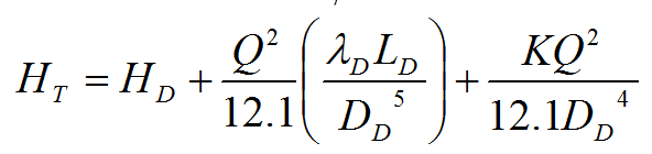
4. For each flow rate, determine the total head H_T: (see note about K in “Supporting Information”)

5. Plot H_T versus Q on the same graph as the manufacturer’s pump performance data (H-Q relationship). Be sure to make the units for Q consistent! Carefully determine the intersection point, and the corresponding predicted flow rate. If necessary, refine the range of flow rates to focus your estimate around the intersection point (e.g. if the two curves do not intersect, you might need to test smaller or larger flow rates than the original range).

6. Record the predicted flow rate as accurately as possible according to the intersection point.

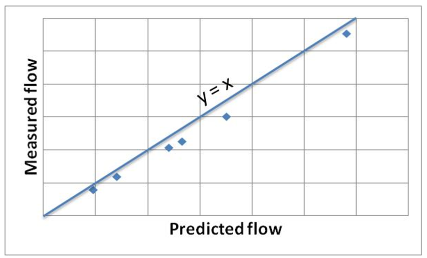
Comparing predicted and observed data

Once you have repeated the above steps for each of the 24 pipe systems, you will have a set of 24 pairs of predicted and observed flow rate. Put these values in a table so that you can plot predicted versus observed flow on a graph and then draw a straight line on the graph corresponding to y = x. Then see how well your points align to the y = x line.

In the example to the left, the predicted values are all to the right of the y = x line, indicating that the predictions are high with respect to reality. The data are well-aligned with respect to each other (minimal random error) so we can have some faith in the test results, but there is a clear systematic error so there must be more loss (e.g. higher minor losses) in the system than was assumed in the calculation.

On the other hand, if the points had been more randomly spread out, but were equally occurring on both sides of the y = x line, then we might assume that the assumptions were satisfactory, but that the practical results were less reliable, and so on.

Assumed values

Surface roughness of poly pipe, k = 0.007 mm

Fluid density, ρ = 1000 kg/m³

Fluid viscosity, μ = 1.005 x 10^-3kg/ms

Note: No suction pipe so we assume no pipe friction losses on the suction side of the pump.

Minor losses

We also need to make an assumption about whether to include or neglect minor losses in our system. There will be minor losses in the pump exit pipe, the sudden contraction to the main delivery pipe, and there will also be the exit loss. Depending on how straight you managed to get the pipe there might be some minor losses along the way as well. You can start out by assuming an overall minor loss coefficient K = 3, but as this parameter is unknown, it can adjusted to account for discrepancies between observed and predicted results.