Practical 4: Pump Performance
| Site: | learnonline |
| Course: | Introduction to Water Engineering |
| Book: | Practical 4: Pump Performance |
| Printed by: | Guest user |
| Date: | Thursday, 30 April 2026, 6:37 AM |
Description
Practical 4: Pump Performance
Introduction
Design of pumped systems involves the careful selection of a pump (or group of pumps) to deliver the required flow rate at the required head. Lack of care can lead to a variety of problems, including pumps delivering insufficient flow, consuming more energy than necessary or causing excessive wear due to operating outside the pump’s “preferred” zone of head or flow.
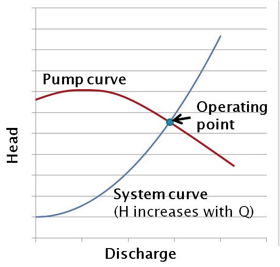
The flow rate delivered in a pumped system is given by the intersection point between two curves: the pump curve and the system curve.
The pump curve
Pumps are built to operate over a specific range of total head (H) and flow rate (Q). The typical H-Q relationship for a pump is a curve connecting two points from a maximum value of H (at which flow Q drops to zero) to a maximum theoretical flow rate Q (at which there is no head H).
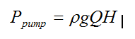
The hydraulic pumping power (Ppump) is given by:
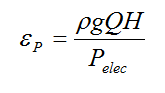
The electric motor driving the pump consumes energy at a rate Pelec, and the resultant efficiency of the motor-pump combined unit is given by:
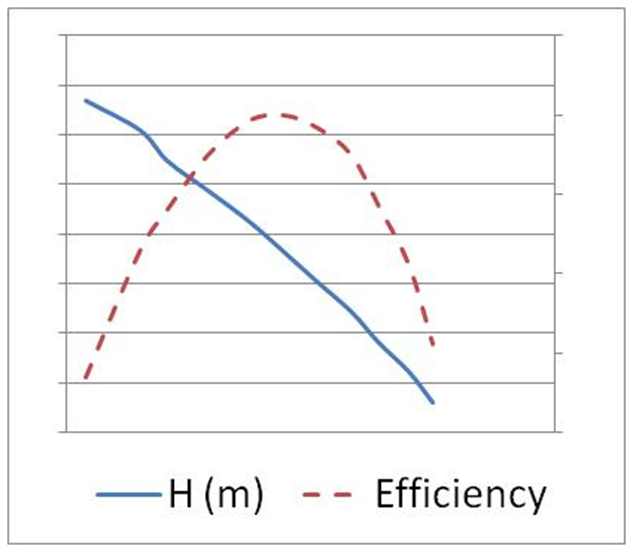
Generally, pumps are designed with a rated head and discharge called the “design point”, corresponding to the specific H-Q combination that gives maximum efficiency (see figure 11.17 below, from Hamill 2011). Pumping at either a higher head (lower flow) or higher flow (lower head) yields sub-optimal efficiency and depending on the pump, the efficiency of pumping away from the rated head and discharge may be extremely low, leading to a great deal of wasted energy.
Supporting Information
The system curve
Like pumps, a pipe system has a distinct H-Q relationship, because as flow increases, friction head losses increase. There is also a “static” (elevation/lift) head component in pumped systems. In low flow, high lift and/or short wide pipe situations the static head may dominate and the total head is not significantly dependent on flow rate. However, for high flow and/or long thin pipelines, the friction head losses can be significant and are heavily dependent on flow rate.
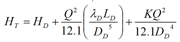
The basic H-Q relationship for a pipe or pipe network is called the “system curve” and the total head HT is given by:
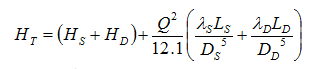
where HS and HD are the static lift (m), and are the Darcy friction coefficients, LS and LD are the pipe lengths (m) and DS and DD are pipe diameters. Subscripts S and D denote the suction and delivery lines, respectively. Note the strong dependence on pipe diameter in this equation. In the equation above, minor losses have been neglected.
For a pumped system, we find the “operating point” by determining the intersection between the pump curve and system curve (see figure, left). This is the head and flow-rate at which the system is expected to operate. Appropriate pump selection involves aligning (as best as possible) the operating point to the pump’s design point.
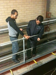
Apparatus
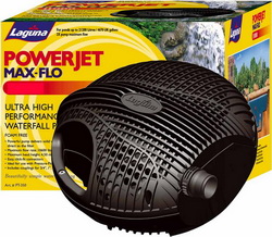
This practical uses a submersible pond pump with maximum head of 3.5m (no flow) and maximum flow of 1.5 L/s (no head), and eight pipes to be shared.
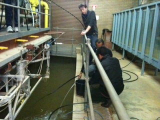
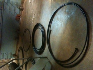
Pipes are standard black polyethylene garden irrigation pipe (k = 0.007mm), in two diameters (13mm and 19mm, internal diameter). For each diameter, there are four lengths (5m, 10m, 15m and 20m) available for testing. This practical makes use of a large rectangular channel sump in the hydraulics laboratory for both the water source and discharge. It could alternatively be adapted to any relatively large body of water, such as a swimming pool, spa or large trough.

Experimental Method
- Select a pipe for testing and carefully screw the fitting to the outlet of the submersible pump.
- Roll out the pipe on the floor alongside the concrete channel sump, so that it is relatively straight, and check that it does not contain “kinks” (where the pipe twists and folds on itself, obstructing flow).
- Carefully lower the pump into the water using a rope tied to the handle (DO NOT support the weight of the pump using either the pipe or the power cord!)
- Hold the discharge end of the pipe at a steady elevation between and measure this relative to the water surface in the sump (aim for elevations between 0.5m and 2m above the water level). Make sure there is enough room available to place a bucket under the end of the pipe.
- Switch on the pump at the power supply and allow the flow in the pipe to reach a steady rate (hint: hold the end over the sump!)
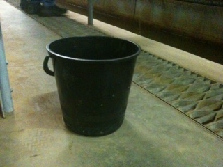
- Using a stopwatch, measure the exact time taken to fill a bucket of known volume. Repeat this several times for the same outlet elevation to reduce the effect of random error. (Flow rate, Q = Volume / Time.)
- Repeat steps 1-6 for each pipe diameter and length combination, trialling different elevations each time. Try to cover a broad range, from high flow (short pipe, large diameter, low static lift) to high head (long pipe, small diameter, high static lift).
Data for Analysis
Please download the spreadsheet to obtain data for this experiment.
As you’ll see, the experiment was run twice for 24 different scenarios – each scenario represents a unique pipe system in terms of the specific combination of pipe length (5, 10, 15 or 20 metres), diameter (13 or 19 millimetres) and static lift (low, medium and high). Multiplying these combinations together (4 lengths, 2 diameters and 3 static lifts) gives the 24 individual scenarios. The parameter being measured was the time taken (seconds) to fill a 10 litre bucket, which you will use to determine a flow rate.
Two tests were done for each scenario – you should use the average value from the two tests but also be sure to inspect each test to see if there are any obvious sources of error (e.g. if there is a large discrepancy between two tests for the same scenario it is an indicator that something went wrong in one of those tests).
Calculations
Introduction to Water Engineering Practicals
Calculations
CalculationsPart 1. Design Point As we were not given a “design point” for this pump, you will need to determine (as accurately as possible) the H/Q combination corresponding to maximum efficiency – we will assume that this is the design point for this pump. You can determine the efficiency of the pump (assuming constant Pelec = 80 watts) for each H-Q combination given in the manufacturer’s pump data, and produce a plot of head and efficiency versus discharge (hint: plot “head” on the primary axis and efficiency on the “secondary axis”). Include these calculations and the graph, plus the resultant design point, in your report. Part 2. Operating Point You need to determine a unique system curve for each pipe system tested (note that a “pipe system” is each unique combination of diameter, length and static lift – so there were 24 such systems altogether). This is most easily done in a spreadsheet program where you can set up the formulas and then simply change the parameters to determine a new system curve. |
Supporting InformationPump DataThe following data is from the pump manufacturer (Note: LPH = litres per hour) Q (LPH) Height (m) 300 3.35 1100 3.05 1500 2.75 2100 2.44 2700 2.13 3200 1.83 3700 1.52 4200 1.22 4600 0.91 5050 0.61 5400 0.30 Power consumption = 80 watts (we assume this is relatively constant, irrespective of H and Q). Assemble the given pump performance data to plot the H-Q performance curve.
|
|
|
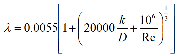
Calculation steps For each combination of pipe diameter, pipe length and static lift, you must determine the whole system curve for an appropriate range of hypothetical flow rates. Therefore you must repeat the following steps for each of the 24 scenarios: 1. Set up an array (list) of flow rates varying from 0.01 to 2 L/s (convert to m3/s) 2. Calculate the velocity and Reynolds number corresponding to each flow rate, for the pipe diameter under consideration 3. For each Re, calculate the Darcy friction coefficient using the Moody equation:
4. For each flow rate, determine the total head HT: (see note about K in “Supporting Information”)
5. Plot HT versus Q on the same graph as the manufacturer’s pump performance data (H-Q relationship). Be sure to make the units for Q consistent! Carefully determine the intersection point, and the corresponding predicted flow rate. If necessary, refine the range of flow rates to focus your estimate around the intersection point (e.g. if the two curves do not intersect, you might need to test smaller or larger flow rates than the original range). 6. Record the predicted flow rate as accurately as possible according to the intersection point.
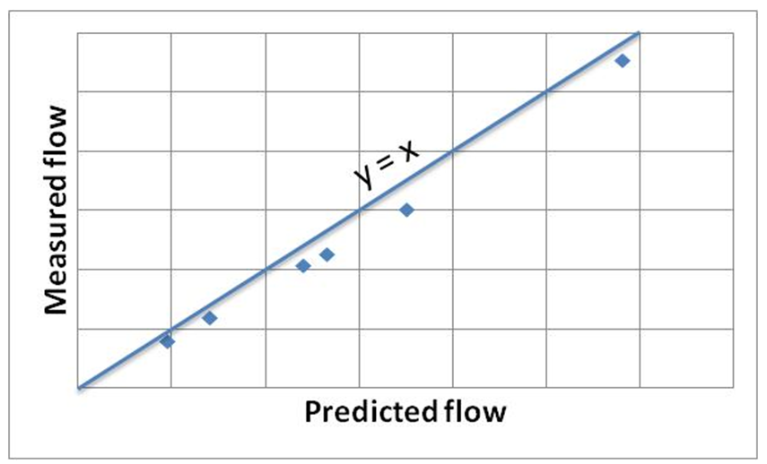
Comparing predicted and observed data Once you have repeated the above steps for each of the 24 pipe systems, you will have a set of 24 pairs of predicted and observed flow rate. Put these values in a table so that you can plot predicted versus observed flow on a graph and then draw a straight line on the graph corresponding to y = x. Then see how well your points align to the y = x line.
In the example to the left, the predicted values are all to the right of the y = x line, indicating that the predictions are high with respect to reality. The data are well-aligned with respect to each other (minimal random error) so we can have some faith in the test results, but there is a clear systematic error so there must be more loss (e.g. higher minor losses) in the system than was assumed in the calculation. On the other hand, if the points had been more randomly spread out, but were equally occurring on both sides of the y = x line, then we might assume that the assumptions were satisfactory, but that the practical results were less reliable, and so on.
|
Assumed values Surface roughness of poly pipe, k = 0.007 mm Fluid density, ρ = 1000 kg/m3 Fluid viscosity, μ = 1.005 x 10⁻³kg/ms Note: No suction pipe so we assume no pipe friction losses on the suction side of the pump. Minor losses We also need to make an assumption about whether to include or neglect minor losses in our system. There will be minor losses in the pump exit pipe, the sudden contraction to the main delivery pipe, and there will also be the exit loss. Depending on how straight you managed to get the pipe there might be some minor losses along the way as well. You can start out by assuming an overall minor loss coefficient K = 3, but as this parameter is unknown, it can adjusted to account for discrepancies between observed and predicted results.
|