MATLAB
| Site: | learnonline |
| Course: | MATLAB |
| Book: | MATLAB |
| Printed by: | Guest user |
| Date: | Tuesday, 5 May 2026, 5:18 PM |
Description
MATLAB Short Course
1. General Information
This book aims to introduce students to a number of the essential concepts of MATLAB.
It is designed to assist the learning of Matlab relevant to the syllabuses for the first year mathematics courses in the Engineering associate degree programs at the University of South Australia.
- Using MATLAB in Calculus by G. Jensen, and
- Understanding Linear Algebra Using MATLAB by E. & M. Kleinfeld.
It is best to read, attempt and fully comprehend the concepts being introduced in this guide before progressing to similar sections in Jensen. However, it is expected that they will complement each other most beneficially.
What is MATLAB?
At the simplest level, MATLAB is a powerful calculator. At the more advanced level, MATLAB is a high-performance language for technical computing. It integrates computation, visualisation and programming in an easy-to-use environment where problems and solutions are expressed in familiar mathematical notation.
MATLAB is an interactive system whose basic data element is an array that does not require dimensioning. This allows you to solve many technical problems related to science and engineering, especially those involving data that can be held in matrices and vectors.
Because MATLAB has been designed around engineering and scientific applications, it requires only a fraction of the time to write a program compared to scalar non-interactive languages such as C or FORTRAN.
Matlab is structured using a large collection of files, called M-files. These are of two quite different types, namely script M-files and function M-files. You can use these M-files to do arithmetic calculations, numerically solve equations, create graphics, etc. You can usethe M-files supplied in MATLAB to build up sophisticated computer programs. But, most importantly, you will need to create and store your own M-files to supplement those already provided by MATLAB in order to solve your specific problems.
By using the Symbolic Math Toolbox, your MATLAB M-files can also include differential and integral calculus, linear algebra, algebraic simplifications, algebraic solution of equations, variable-precision arithmetic, etc.
Logging on and off
MATLAB is available in UniSA's OUA Lab Virtual desktop. It is remotely possible that MATLAB might be temporarily unavailable on times of maximum usage by other students. Log onto the VDI using the client installed on your machine using your UniSA log in.
In the Applications folder is MATLAB. Double click this icon. The default Matlab Desktop Layout which appears is shown at the back of this guide. In the “Command History”, you can view previously used functions, and can copy and execute selected lines. However, the “Command Window” is the most important, and this is where you enter variables and commands, and where you define functions and run M-files.
We suggest you opt to expand this window by clicking on “View”, followed by “Desktop Layout” and then choosing “Command Window Only”. You can always bring back the other windows later by choosing “Default” under “Desktop Layout”.
In Command Window, you will see “>>”: >> is the MATLAB prompt. When the Command Window is the active window, a cursor should appear to the right of this prompt, indicating that MATLAB is waiting to answer a mathematical query or execute a command.
When you have finished your MATLAB session, and saved on your flash drive everything that you wish to save, you need to exit from MATLAB and the virtual desktop. To do this, enter either the command quit or exit after the prompt, or else click File followed by Exit Matlab. Then logoff of the VDI.
Getting Help
If you experience any technical difficulty accessing or using MATLAB, please contact UniSA's IT helpdesk on 8302 5000
Managing multiple windows
Quite often while using MATLAB you will have a number of windows in operation simultaneously.
For example, you might have the MATLAB Command Window, a couple of windows containing M-files you have constructed, at least one window containing graphical output, and even a Microsoft Word window where you have copied output in preparation for the final printed report.
You can reduce an individual window to an icon on the bar at the bottom of the screen, out of the way, and can retrieve it later on. Each window has some grey buttons at the top right-hand corner with symbols on them. If you wish to move a window out of the way temporarily, click on the left button with a ’-’. It can be recalled later by clicking on the corresponding icon on the bar at the bottom of the screen. The centre button increases or decreases the size of the window. The right button, with an ’x’, removes the window totally.
Some windows may get in the way of the icons. We assume you know how to use the mouse button to move windows around the screen.
Working with a Flash drive
While you are working in the VDI, any files that you create which need to be accessed should be saved on to the VDI's hard drive. However, at the end of a session, when you log off the computer, you will lose all such files that you have saved unless you save them to disk or flash drive.
Soon you will be constructing M-files. These will be explained in more detail later, but previous information has already signalled that there are two quite different types, namely script M-files and function M-files. A script M-file will contain a sequence of MATLAB commands designed to solve a particular problem. A function M-file is of a different form, and enables you to extend the list of standard MATLAB functions by constructing, naming and saving your own functions.
As long as you are in the MATLAB environment you can access all of the M-files which constitute the professional version no matter on which disk drive or flash drive you are working. However, if you need to access an M-file which has been stored on a floppy disk or flash drive, you must change your working directory to that drive. After the >> prompt, type in cd a: (or another letter, instead of a, for the appropriate drive) which changes the directory to the a: drive (the flash drive). Then, to get a list of the files that are stored on the disk or flash drive, you can enter dir after the prompt.
Saving M-files to a storage device
Let us assume you have an active window (such as the M-File “Editor/Debugger” window) containing an M-file, and you have placed a disk in the disk drive.
Click on File, then on Save As....
In the Save in: box, specify the location where you want this M-file saved. If you merely wish to save it during this session, you must specify the e: Scratch drive on the computer.
If you wish to save it on your flash drive, you need to choose the a: or another appropriate drive.
In the File name: box, you must enter the name you have chosen for this M-file. All MATLAB M-files must have names that finish with .m such as test1.m or project.m or myfunctn.m or prac3wk8.m, etc. NOTE: every year some students cause all sorts of anguish to themselves by selecting a name for their M-file which happens to already be the name of one of MATLAB ’s own M-files. This must not be done! For example, do not name your M-file sin.m because this is where the trigonometric function sin x is stored in MATLAB. Never name your M-file solve.m because that is the name of a file in the Symbolic Math Toolbox which solves an equation. As there are hundreds of M-files in MATLAB, you need to be careful when naming your own.
Once you have selected a name, click on Save.
Thereafter, if you make any changes to this M-file, and you need to save those changes, you click on File, then on Save in the “Editor/Debugger” window. Alternatively, you could click on the “Save” icon.
Loading M-files from a storage device
After the MATLAB prompt, change directory to the floppy. Type in dir just to check what is on the floppy disk or flash drive. Click on File, then Open and double click the required M-file. This will open the file inside the “Editor/Debugger” window where additions and corrections can be made, and later saved as described above.
2. Simple Mathematics
You can use MATLAB as a calculator. Firstly, we will perform simple arithmetic using the operations + (addition), - (subtraction), * (multiplication), / (division), ^ (raise to a power, or exponentiation). We will also include parentheses (brackets).
Enter the MATLAB Command Window. Type in each of the following arithmetic expressions after the >> prompt and press the Enter key at the end of each line. Before doing so, mentally calculate the answer you expect to see in each case.
(7+6)/(10-2)
7+6/(10-2)
7+6/10-2
9+(6*2)/(3*4)
9+6*2/(3*4)
9+6*2/3*4
1.00001^100000
You will notice that the last expression is very close to the exponential number e. This will be explained later in lectures.
Some students are unsure of the use of parentheses (brackets). They often use many unnecessary brackets, thereby making expressions hard to interpret. But other students omit brackets when they are absolutely needed. The order in which these operations are evaluated in a given expression is given by the usual rules of precedence, which can be summarised as follows:
| Expressions are evaluated from left to right, with the power operation having the highest order of precedence, followed by both multiplication and division having equal precedence, followed by both addition and subtraction having equal precedence. Brackets can be used to alter this usual ordering. |
Variable names
You would have noticed that MATLAB gives the result of each calculation the default name ans. This clearly will become confusing and unacceptable when a sequence of commands is executed, especially in an M-file. Hence, you should always give the result a variable name. This variable name can then be used in subsequent calculations in a manner similar to putting a result in the memory of a calculator. The rules for variable names are
- variable names are case sensitive; crows, Crows, cROWs, CROWS are all different variables
- variable names can contain up to 63 characters; prideofsouthaustralia is acceptable
- variable names must start with a letter, followed by a mixture of letters, digits or underscores. Other symbols and spaces are not allowed; x, ABC, item3week1, profit_1999, Pride_of_South_Australia are all acceptable variable names
Type in the following sequence of commands after the prompts on consecutive lines
x=7.231
y1=x+1/x
y2=x-1/x
difference=y1^2-y2^2
Exercise: explain why the answer must be 4 for any initial x. Then use the up-arrow repeatedly to change x to any other non-zero value, find new y1, y2 and demonstrate that difference is always 4.
Note: this continual use of the up-arrow will become unmanageable and very confusing when we have a longer sequence of commands. That is where the use of M-files will become crucial.
Comments, clear, ; and Ctrl-C
Comments using % sign
All text after a percent sign (%) is taken as a comment statement and is simply ignored by MATLAB. It helps you and readers understand what certain variables represent or what outcomes your commands are trying to achieve.
Clear previous variables
If you have been working with MATLAB in a long session you may wish to re-use a variable name for a different purpose. This is especially important if, say, you had an array variable x and now you want to use x for a scalar variable or a shorter array x. Then you can delete the previous variable from the MATLAB workspace using the command clear x.
You can also delete all variables no longer required using clear all. This is useful if you are starting a new problem .
Suppress output
A semicolon (;) after a calculation command tells MATLAB to suppress the result. When you have a large amount of data, or certain variables are not needed to be shown in the final output, they need not be displayed. They will still be held in memory ready for future use. For example, suppose you want to know where the straight line passing through the points (x1, y1) = (3, 4) and (x2, y2) = (8, 7) intersects the y-axis. Type in the following commands:
clear all
x1=3, y1=4
x2=8, y2=7
%let m be the slope of the line y=m*x+b
m=(y2-y1)/(x2-x1);
% y-y1=m*(x-x1) intersects y-axis when x=0
% this gives b=y1-m*x1
y_intercept=y1-m*x1
Exercise: add a command to find where the straight line intersects the x-axis.
Exercise: You know that two points on the curve  are x1 = π/6 , y1 = 1/2 and x2 = π/3, y2 = √3/2. In MATLAB , pi represents the number π while sqrt(3) represents the number √3.
Use the up-arrow to change the commands above to find the intercepts on both axes of the straight line joining these two points.
Ctrl-C
Sometimes you will inadvertently set MATLAB into a never-ending loop or cause masses of numbers to scroll down the screen. You can interrupt MATLAB at any time by pressing Ctrl-C.
Elementary Maths
All of the mathematical functions on your calculator are available in MATLAB , as well as many other elementary functions. To view a list of the common functions, click on “Help” at the top of the MATLAB Command Window, then click on “MATLAB Help”, and then double click on MATLAB Functions Listed by Category. Then click on Elementary Math Functions.
(Note there are also Specialized Math Functions beyond the scope of this introduction.)
For brief information about any of the elementary functions, merely double click on that function name. You can use the back-arrow near the top of the window to move back to previous windows. Of special significance, note there are the six trigonometric functions as well as their corresponding inverse functions. For example, the MATLAB expression sin(x) represents sin x. Note the use of brackets around the x. Of course, MATLAB only uses natural radian measure and never degrees. Type in the following (non-comment) commands:
theta=3*pi/4
y1=sin(theta), y2=cos(theta), y3=tan(theta)
% note than you can put more than one command on a given line,
% separated by commas. Now find the reciprocal of each:
z1=csc(theta), z2=sec(theta), z3=cot(theta)
% Find alpha, beta such that sin(alpha)=0.721 and tan(beta)=-1.78
alpha=asin(0.721), beta=atan(-1.78)
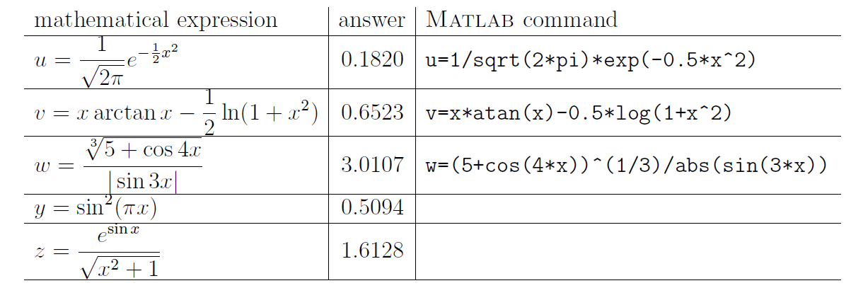
There are also the six hyperbolic functions and their inverse functions, to be discussed later in Chapter 6 of Grossman. Of special importance, note that
- the exponential function ex is represented in MATLAB by exp(x)
- the natural logarithm function ln x is represented in MATLAB by log(x)
- the square-root function √x is represented in MATLAB by sqrt(x)
- the absolute value function |x| is represented in MATLAB by abs(x)
Exercises: Let x = 1.253. Show that the variables u, v, w, y, z have the values shown by typing in the corresponding MATLAB commands:
Other Useful Functions
round(x) rounds x to the nearest integer
floor(x) rounds x down to the nearest integer
ceil(x) rounds x up to the nearest integer
rem(y,x) the remainder after dividing y by x
sign(x) =−1 if x< 0 ; =0 if x=0 ; =1 if x> 0
rand generates a random number between 0 and 1
Exercise
You have $50. Each item costs $3.35. How many items can you buy and how much change will you have left?
number_of_items=floor(50/3.35)
% change default format to one with two decimal places
format bank
change=rem(50,3.35)
Note: to view other possible formats, type in help format after the MATLAB prompt.
Exercise: There are 211 students to be arranged into tutorial classes which can hold 24 students per class. Use MATLAB commands to determine the number of tutorial classes needed and how many spare places are left.
Assignment statements
The preceding MATLAB commands that assign the value of the expression after the ’=’ sign to the variable before the ’=’ sign are assignment statements. Note that all variables in the expression after the ’=’ sign must have previously been allocated a value, or else an error occurs. For example, enter the following commands:
a=3
B=4
c=sqrt(a^2+b^2)
You will see the error message ??? Undefined function or variable ’b’. Consider the following:
clear all
x=7
x=x^2-12
The last line has nothing at all to do with a mathematical equation. It is a MATLAB assignment statement that calculates x2 −12 at x = 7 and stores the result in the variable x, thereby over-writing the previous value.
3. Script M-files
As has been mentioned already, for simple problems it is easy to enter your requests after the prompt in the MATLAB Command Window. However, as the number of commands increases or whenever you wish to make major changes, this becomes very tedious. Instead, you should place MATLAB commands in a simple text file, and then tell MATLAB to open the file and evaluate all the commands precisely as it would if you had typed them after the prompt. These files are called script M-files and must have filenames ending with the extension ’.m’. Examples of possible M-file names are example1.m, proj1Y2000.m, question5.m, mechdevice.m, etc.
Using M-files
To create a script M-file, click on “File” in the MATLAB Command Window, then on “New” followed by “M-file”. This opens the M-file “Editor/Debugger” window, where you can enter your sequence of MATLAB commands, in simple text format without any prompts. As a first example, reconsider the problem of finding the intercepts on the axes this section. Type in the following:
clear all
x1=3
y1=4
x2=8
y2=7
%let m be the slope of the line y=m*x+b
m=(y2-y1)/(x2-x1);
% y-y1=m*(x-x1) intersects y-axis when x=0
% this gives b=y1-m*x1
y_intercept=y1-m*x1
x_intercept=x1-y1/m
Now save this file as described earlier. Save to your flash drive. You will note that the header now shows the directory location as well as example1.m as the name of this M-file.
Return to the MATLAB Command Window and enter example1 after the prompt. Assuming you have changed to the same directory, this will execute the sequence of commands in example1.m.
Return to the “Editor/Debugger” window. Use the mouse, arrows, backspace and delete facilities to change x1,y1,x2,y2 to the values specified in the second exercise in this Section. Then Save and again enter example1 after the >> prompt. Of course this can most simply be accomplished using the up-arrow once.
Search Path
Suppose you type in crow after the prompt; in other words >> crow
How is this to be interpreted? MATLAB interprets this statement using the following hierarchy:
- It checks to see if you merely wish to print out the value of a variable named crow in the current MATLAB workspace. If not,
- it checks to see if crow is a built-in MATLAB command. If not,
- it checks to see if you wish to execute an M-file named crow.m that you have saved in your current working directory. (There is a further possibility not discussed here.)
Revision Exercises
Exercise 1: Suppose you want to find the two zeros of the quadratic ax2 + bx + c. (As you would expect, Matlab already has a procedure to do this automatically, but let us solve this independently.) Firstly, to solve 5x2 −17x−12 = 0, you should create, save and execute an M-file quadzeros.m (for example)
clear all
a=5, b=-17, c=-12
x1=(-b+sqrt(b^2-4*a*c))/(2*a)
x2=(-b-sqrt(b^2-4*a*c))/(2*a)
Then change this to find the zeros of each of the quadratics
3x2 + 5x − 13 2x2 − 7x + 23 2.34x2 + πx − √6
Exercise 2: Suppose the three sides of a triangle have lengths (in cm) a = 11.7, b = 6.9, c = 7.1. Find the three angles A,B,C using the cosine rule
a2 = b2 + c2 − 2bc cosA
and the sine rule
a/sinA = b/sinB = c/sinC
Convert the angles into degrees.
Construct the following in an M-file triangle.m, and then execute it.
clear all
a=11.7; b=6.9; c=7.1;
% let cA represent cos(A), and sB represent sin(B)
cA=(b^2+c^2-a^2)/(2*b*c);
A=acos(cA);
sB=b*sin(A)/a;
B=asin(sB);
C=pi-A-B;
% convert angles into degrees for output
A=A*180/pi; B=B*180/pi; C=C*180/pi;
fprintf(’angle A is %6.2f degrees \n’, A)
fprintf(’angle B is %6.2f degrees \n’, B)
fprintf(’angle C is %6.2f degrees \n’, C)
You will notice that the fprintf command produces neat output. In each case, the variable to be printed is at the end, while %6.2f stipulates where the value is to be printed along with how many positions (6) and how many decimal places (2). The \n moves to a new line after printing whatever precedes it, in preparation for more output.
Exercise 3: Consider the two simultaneous linear equations
a11x + a12y = b1
a21x + a22y = b2
MATLAB provides various ways to solve this automatically, given values for the coefficients, as we shall see later. But for now, you will write your own M-file. You will need to give values for the four coefficients and the numbers on the right hand side, find  = a11a22 − a12a21 so that
x = a22b1 − a12b2 / detA and y = a11b2 − a21b1 / detA
providing detA ≠ 0. Test your M-file on the following two problems:
2x − 3y = 2 3x − 11y = 17
5x + 6y = 59 −6x + 22y = 23
The solution of the left system is x = 7, y = 4. The right system clearly does not have a solution.
Entering Long Expressions: if an expression does not fit on a single line, use three dots . . . to indicate that the statement continues on the next line. Do not leave any unnecessary blank spaces and press Enter or Return immediately to advance to the next line, and continue entering the statement. Be careful to create this break at a sensible point in the expression, preferably after a comma or mathematical operation.
4. Arrays
All of the computations considered so far involve single (scalar) numbers. One of the powers of MATLAB is its ability to do computations on arrays, where the same operation is performed on all numbers in a data array using a single command. Special types of arrays such as matrices and vectors will be discussed in more detail in Section 9, as will mathematical operations specific to them.
Constructing Arrays
We will illustrate four somewhat different ways of constructing a simple array of numbers. The whole array is represented by a variable name along similar lines to scalar variables. For example, a, x, Y, A3, Xarray are suitable names for arrays providing they have not already been used for another purpose. The first method of constructing an array is merely to list the numbers in the array, enclosed inside square brackets and divided either by spaces or commas. Type in the following after the prompt:
x=[3, -5.1, 0, 6, 11, -17, pi]
y=[8 2 -12 3/4 1.234567 1 10]
This is fine if you have only a few numbers to input into an array (seven in each of the above two examples). However, if there are hundreds, we need another method. This is possible if the numbers in the array are equally spaced. We use the colon notation. Type in the following after the prompt:
A=[-3:21]
B=[3.33:12]
Clearly [a:b] is an array starting at a with increments of one until we reach b but not going beyond b. If a and b are integers with a < b, the number of elements in the array is b − a + 1. Why?
Suppose we want an array to extend over the interval from a to b with n equal subintervals of length h. Then clearly h = b − a/n and the number of elements in the array will be n + 1. Why?
For example, suppose you wanted an array of values from 2.5 to 4.0 with 25 subintervals, which implies that the values need to be incremented by a step-size of h = 0.06. Why? The number of values in the array will be 26. Show that the following three expressions are equivalent by entering each expression (Matlab command only) after the prompt:
C=[2.5:0.06:4.0] [a:h:b] is an array from a to b with step-size h.
C=linspace(2.5,4.0,26) linspace(a,b,n+1) is an array from a to b with n subintervals, n + 1 points (avoids having to find h).
C=2.5 + 1.5*[0:0.04:1] divides the interval from 0 to 1 into 25 equal subintervals of length 0.04 and then scales & shifts.
Which of the above do you prefer?
Of course, when you have an array with a large number of elements you should follow statements like those above with a semi-colon “;” to avoid printing lines of probably unwanted numbers in your output.
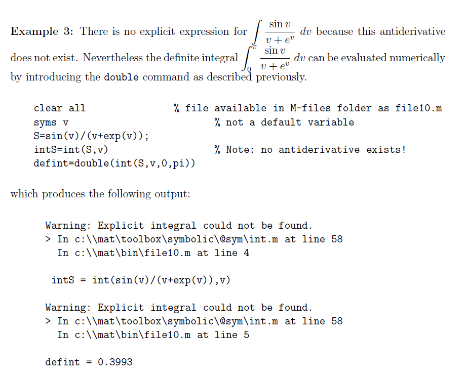
Example 1:
An array from −2π to 2π using 150 subintervals is
array1=linspace(-2*pi,2*pi,151);
Example 2:
An array from 3 to 76 with steps of 0.5 is
array2=[3:0.5:76];
Exercise: Suppose we need an array (in hours) to represent the 24 hours of a day, from midnight to midnight, and we want to have time-steps of one minute. Then a suitable array might be:
day=[0 : 1/60 : 24];
What equivalent statement uses the linspace command?
You can append the elements of one array to the end of another array. Enter the following:
clear all
x1=[1 6 -7]
x2=[5 9 0 -1 11]
x=[x1 x2]
Array Subscripts
Given an array, you may need to access only one or some of the individual elements contained in the array, rather than the whole array itself. If A is an array with n elements in it, and i is an integer such that  ≤
≤  ≤
≤  , then in Matlab A(i) is the th element in the array (often denoted by Ai in mathematics).
To illustrate this, enter the following into an M-file and then execute it. Firstly you will construct an array containing 9 random numbers between 0 and 1. Then you will use these elements of A to introduce scalar variables or new arrays which are merely sub-arrays of A. In each case the new variable names before the “=” signs have been suggested so that you can read the output conveniently. Please study carefully the expressions following the “=” signs as they are commonly used.
A=rand(1,9)
% the next two lines define scalar variables
a1=A(1)
a7=A(7)
% the remaining lines define new arrays
a3456=A(3:6)
a1357=A(1:2:7)
a852=A(8:-3:2)
Exercise 1: After executing the above M-file, what would you expect to see if you now entered each of the following after the prompt? Because we have not allocated a variable name for either expression, both of course will be named ans by default.
a852(3)
a1357(2:3)
Exercise 2: The MATLAB command
Q=linspace(0,100,141);
creates an array which has 140 subintervals and 141 points. Print out only
- the 46th element of Q
- the first four elements of Q
- the last three elements of Q.
Special array functions: sum, prod, length, max, min, sort, find, diff
The functions sum, prod, length, max, min, sort, find of an array are self explanatory by creating and executing the following in an M-file (do not type in the comment statements). diff(Z) is a new array containing the differences between consecutive elements of Z.
clear all
% create an array with 11 elements,
% each of which is a random number between 0 and 5
Z=5 * rand(1,11)
Zsum=sum(Z)
Zprod=prod(Z)
Zlength=length(Z)
% ’max’ finds the maximum value and its subscript (index) number
[Zmax,i] = max(Z)
[Zmin,j] = min(Z)
% ’sort’ and ’find’ create new arrays
Znew=sort(Z)
Zbig=find(Z>3.0) % for example, finds subscripts where Z(i) is >3.0
Znewbig=find(Znew>3.0) % have now moved to end of array
Calculating
Performing arithmetic calculations on arrays containing large data sets is considerably easier with MATLAB than with other computer languages such as C or Pascal. It is precisely the ease of array manipulation that makes MATLAB suitable for mathematical, scientific and engineering applications.
Basic arithmetic operations on arrays
If X is an array and a, b are scalar values, then a∗X+b creates a new array by multiplying all the elements of X by a and then adding b to each position. What do you expect X/a+b to give?
Enter X=[1:8] after the prompt. Then execute
y=10*X+7
z=(y-7)/10 %why is this the same as X?
v=3*X/2 -1
If A,B are two arrays containing the same number of elements and c1, c2 are scalars, then expressions of the form c1A ± c2B will create new arrays. Enter the following:
clear all
A=[1:2:11] , B=[8:-1:3]
C=B-A
D=(3*A-4*B)/2 + 5
However, there are some other very important differences. Later you will see that MATLAB includes standard operations with matrices and vectors, which are also examples of arrays. Hence, to distinguish those operations, a dot must be placed immediately before the ∗ / ^ operators in each of the following circumstances, where A,B are arrays of the same length and c is a scalar.
A .* B A ./ B c ./ A A .^ B c .^ A A .^ c
In other words, a dot is required before the operator whenever two arrays are multiplied together, whenever you divide by an array, and whenever an array occurs in any power expression. These always create a new array of the same length as A (and B). Enter the following and take careful note of the answers:
clear all
X=[1 2 3 4] , Y=[-1 4 2 1/2]
K1=X.*Y % multiply the corresponding elements
K2=X./Y % divide the corresponding elements
K3=5./Y % divide 5 by each element of Y
K4=X.^Y % raise the numbers in X to the corresponding power in Y
K5=2.^X % raise 2 to the power of each number in X
K6=Y.^3 % cube each element in Y
Example 1: Create an array curo that contains the cube roots of all integers from 24 to 30.
clear all
A=[24:30];
curo=A.^(1/3) % note the dot and brackets
Rather than introducing the array A at all, this could be done immediately using
clear all
curo=[24:30].^(1/3)
Example 2: What is the value of the sum
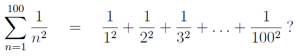
Enter the following:
clear all
% create an array n
n=[1:100]; % note the semi-colon (do not print out the 100 values)
b=1./n.^2; % note the two dots (and the semi-colon)
total = sum(b) % you should get total = 1.6350
Or you could be clever and find this total without actually introducing the array names n, b.
clear total
total = sum([1:100].^(-2)) % note the dot as [1:100] is an array
Exercise: Consider the 40 values n7/2n for n = 1, 2, 3, . . . , 40. Use MATLAB ’s max function to determine the largest of these values and the number n for which it occurs. You should obtain that it is the 10th value equal to 9.7656e+003 which you must know is scientific notation for 9765.6.
Using mathematical functions on arrays
Given an array X and a function f, then the MATLAB command Y=f(X) produces a new array Y such that the elements of Y are Y (i) = f(X(i)) (or in mathematics Yi = f(Xi)). This, coupled with the basic arithmetic operations on arrays discussed earlier enables powerful but simple data manipulation.
Example 1: Enter the following into an M-file and then execute it.
clear all
X=[0:pi/6:2*pi]
Y=sin(X)
Z1=1-2*Y.^2 % note the dot
Z2=cos(2*X) % why are Z1 & Z2 equal?
Example 2: Consider the values tan2(m) for m = 1, 2, . . . , 200. How many of these values are greater than 100?
clear all
m=[1:200];
b=tan(m).^2; % note the dot
c=find(b>100) % finds the positions, not the actual values
number=length(c) % answer is 13 values
Example 3: You should know the classic limit lim x→0 sin x/x = 1. Demonstrate this by evaluating sin x/x for each of x = 0.1, 0.01, . . . , 0.00000001.
clear all
format long % use 16 characters for each value
x=0.1.^[1:8] % note the dot because [1:8] is an array
y=sin(x)./x % note the dot because x is an array
Exercise: The output from an engineering system is y = t2e−t sin t for t ≥ 0. We want to find the maximum value which certainly occurs within 0 ≤ t ≤ 3. Although MATLAB has other more efficient ways of doing this (see later), you could merely investigate this function by dividing the interval [0,3] into 10,000 subintervals (10,001 points). Fill in the missing code in the second and third lines in the following M-file, recalling that the exponential function ex is exp(x) in MATLAB . You should obtain ymax=0.5239, posn=5759, time=1.7274.
clear all
t=linspace( , , );
y= ;
[ymax,posn]=max(y) % use array max function
time=t(posn) % finds corresponding value in the t array
Plotting Graphs
In this section we will use MATLAB ’s plot command to produce graphs. In Sections 6 and 8 you will see there are two other commands to create graphs, namely fplot which uses function M-files and ezplot which is inside the Symbolic Math Toolbox.
If x = {x(1), x(2), . . . , x(n )} and y = {y(1), y(2), . . ., y(n)}, then the MATLAB command plot(x,y) opens a graphics window, called a Figure window, scales the axes to fit the data, plots the points (x(1), y(1)), (x(2), y(2)), . . . , (x(n), y(n)), and then graphs the data by connecting the points with straight lines. If a Figure window already exists, another plot command clears the current Figure window by default (unless instructed not to do so) and draws a new plot. Type in the following as an attempt to graph y = sinx for 0 ≤ x ≤ 2π. [You could replace the last two lines with plot(x,sin(x)).]
clear all
x=linspace(0,2*pi,11);
y=sin(x);
plot(x,y)
Clearly this attempt is unacceptable because we have not used sufficient points! Change the 11 to 201 and execute the code again.
In general, most graphs can be satisfactorily plotted using arrays of, say, 101 to 201 points, although erratic or wildly fluctuating functions would require many more points. Please note that you only need two points to plot a single straight line. For example, to plot a straight line from the point (1,7) to the point (3,-5) you need the command plot([1 3],[7 -5]).
Note: Students often get this wrong by forgetting that the first array always contains the x-coordinates, not the two coordinates of the first point. Similarly, the second array contains the y-coordinates.
Exercise 1: Plot the graph of y = xex/x2 − π2 for −3 ≤ x ≤ 2 using a step-size of 0.02. You will need three dots in the expression to generate the array y.
Exercise 2: Plot the graph of y = sin9x + sin10.5x + sin12x for −π ≤ x ≤ π using 601 points.
Plotting several graphs on the same axes
Example 1: Suppose you want to plot the oscillations y1 = cost, y2 = cos3t and their sum y3 = y1 + y2, for 0 ≤ t ≤ 4π, on the same axes. Here t is measured in seconds and y1, y2, y3 are measured in cm.
clear all
t=linspace(0,4*pi,201);
y1=cos(t); y2=cos(3*t); y3=y1+y2;
plot(t,y1,t,y2,t,y3)
You notice that we found the three y-arrays in a single line of code and they were plotted in different colours. But the empty space at the right end of the graphs is annoying, and how can we label the output so that each graph can be identified? There are many facilities provided by MATLAB to assist you in producing attractive, meaningful graphs. Change the above M-file to the following (this is important!):
clear all
t=linspace(0,4*pi,201);
y1=cos(t); y2=cos(3*t); y3=y1+y2;
axis([0 4*pi -2 2]) % specifies the axes limits
hold on
plot(t,y1,’b--’,t,y2,’g:’,t,y3,’r’)
legend(’y1=cos(t)’,’y2=cos(3*t)’,’y3=y1+y2’)
plot([0 4*pi],[0 0],’k’) % adds the t axis in black
xlabel(’time in seconds’)
ylabel(’displacement in cm’)
title(’oscillations’)
hold off
A short diversion
To get assistance with the MATLAB commands featured above and in the next example, you can use the help facility. Enter each of the following after the >> prompt and carefully read the information until you understand precisely what each of the lines in the previous (or next) M-file is accomplishing.
- help axis
- help plot
- help hold
- help legend
- help text
- help print a menu of print options for your Figure
Alternatively, if you do not know the precise name of a MATLAB command for which you need help, you can click on the Help button at the top of the MATAB Command Window, then click on “MATLAB Help” followed by “MATLAB Functions Listed by Category” and then on a topic of interest. For example, to get help on many graphics related commands, click on Plotting and Data Visualization.
Another help option is the lookfor facility. Suppose you were interested in commands involving the use of complex numbers. After the >> prompt enter lookfor complex.
Example 2: By using hold on and hold off, you can plot several functions on the same axes using a number of plot commands. The functions f(x) = x2 and f−1(x) = √x are inverse functions for x ≥ 0 and hence their graphs must be reflections through the line y = x. Execute the following M-file, carefully noting the results of each command:
clear all % file available in M-files folder as file1.m
axis([0 4 0 4]), axis square
hold on
x1=linspace(0,2,101);
y1=x1.^2; % note the dot
plot(x1,y1)
x2=linspace(0,4,101);
y2=sqrt(x2);
plot(x2,y2)
plot([0 4],[0 4],’k:’) % dotted line in black from (0,0) to (4,4)
text(1.5,3.5,’y=x^2’)
text(3.1,1.7,’y=sqrt(x)’)
grid on % adds grid lines if you want them
title(’reflection property of inverse functions’)
Zoom on
MATLAB provides an interactive tool to expand sections of a plot to see more detail. This is particularly useful if you need to obtain accurate information about where two graphs intersect, or to find the coordinates of an extreme point. The command zoom on, either in your M-file or after the >> prompt turns on the zoom mode. Then go to the Figure window, place the pointer where you want an enlargement and click with the left button. Continue this process and you can zoom in to obtain three or four decimal place accuracy.
Example: Suppose you want to find graphically the point of intersection of y = tanx and y = 1− x3. (Note that there are other non-graphical ways of doing this, described in Sections 6 and 8.) Firstly, plot both of these functions on the same axes for −1.2 ≤ x ≤ 1.2, with at least 800 points to enable zooming. You might also like to add the x and y axes to obtain a figure similar to that on the previous page. Enter the command zoom on. Then zoom in at the point of intersection until you are able to find its coordinates to the accuracy of (0.6376 , 0.7408).
Exercise: Plot y = 10e−t sin t for 0 ≤ t ≤ 2π and then use zoom on to find its maximum value.
Creating separate graphs in one M-file
If you want two separate Figures to be created in one M-file, you can use the figure(n) command where n is a number associated with the window and precedes the set of plotting
commands.
Example: At time t seconds, t ≥ 0, a moving point has coordinates x = sin2t, y = cos3t (metres), and so its speed is given by
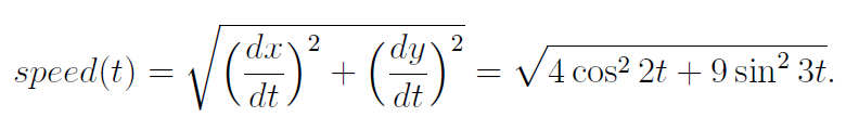
Plot the path taken by the point over one cycle 0 ≤ t ≤ 2π, where t is regarded as a parameter, and also plot the speed against time. Use the following M-file. (You can add your own labels, etc.)
clear all % file available in M-files folder as file2.m
t=linspace(0,2*pi,500);
x=sin(2*t);
y=cos(3*t);
figure(1)
plot(x,y)
axis equal % same scale (metres) on each axis
speed=sqrt(4*cos(2*t).^2+9*sin(3*t).^2); % note the dots
figure(2)
axis([0 2*pi 0 4])
hold on
plot(t,speed)
hold off
5. Control Loops for, while if
MATLAB, along with other computer programming languages and programmable calculators, offers features that allow you to control the sequencing and execution of commands by incorporating decision making facilities. The while and if commands are often used in conjunction with the relational operators.
| Relational Operator | Mathematical Meaning |
| < | less than < |
| <= | less than or equal to ≤ |
| <= | less than or equal to ≤ |
| > | greater than > |
| >= | greater than or equal to ≥ |
| == | equal to = |
|
~= |
not equal to = |
for Loops
A for loop allows a group of commands to be repeated a fixed predetermined number of times. It is typically of the form
for variable=start:step:finish
commands .......
................
end
Note that variable is not an array variable, but a scalar variable that runs through all the numbers in the array start:step:finish one at a time.
Example 1: Calculate the following using both (i) arrays and (ii) for loops:
1 + 1.1 + 1.2 + . . . + 3 and 1 × 1.1 × 1.2 × . . . × 3
(i) clear all (ii) clear all
x=[1:0.1:3]; s=1;
total=sum(x) p=1;
product=prod(x) for t=1.1:0.1:3
s=s+t ; p=p*t ;
end
total=s
product=p
Example 2: Write a simple M-file to produce the following graphic. Use the fact that x = cos(t), y = sin(t), 0 ≤ t ≤ 2π, is the (assumed known!) parametric representation of the unit circle centred at the origin.
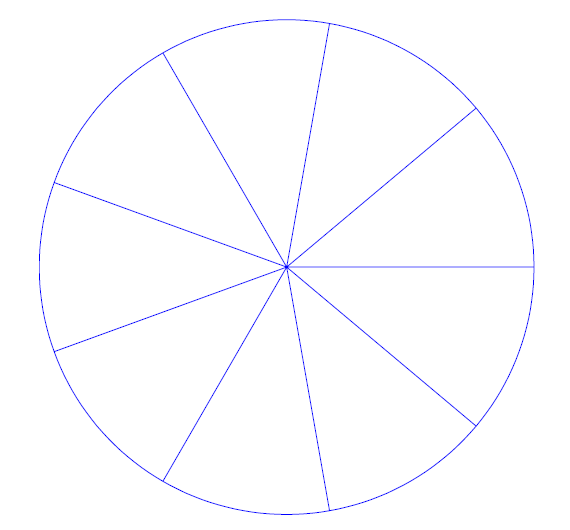
clear all
t=linspace(0,2*pi,181);
% use 181 points to plot circle
x=cos(t); y=sin(t);
plot(x,y)
axis equal, axis off
hold on
for i=1:20:161
% each line needs 2 x-values and 2 y-values only
plot([0 x(i)],[0 y(i)])
end
hold off
Example 3: Suppose you wish to construct a table of values which converts degrees C into degrees F using the standard formula F = 1.8C + 32 for C = 25, 26, 27, . . . , 40.
clear all
fprintf(’ deg C \t deg F \n’) % \t leaves space \n goes to new line
for C=25:40
F=1.8*C+32; % do not print yet, use fprintf instead to line up
fprintf(’%4.0f \t %5.1f \n’,[C F])
end
while Loops
A while loop allows a group of commands to be repeated an indefinite (unknown) number of times until an expression becomes false (is no longer satisfied). It is typically of the form
while expression
commands .......
................
end
The commands between the while and end statements are executed as long as all elements in expression are satisfied.
Example: For what value of n does the summation
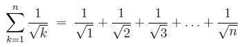
first exceed 30?
clear all
s=0;
k=0;
while s<30
k=k+1;
s=s+1/sqrt(k);
end
number_of_terms=k
sum=s
if-else-end Constructions
The simplest form is
if expression
commands evaluated if expression is true
end
but could be of the more detailed form
if expression1
commands evaluated if expression1 is true
elseif expression2
commands evaluated if expression2 is true
elseif expression3
commands evaluated if expression3 is true
.....................
else
commands evaluated if no other expression is true
end
Example 1: Let us consider a very simple situation firstly. Suppose a shop offers a 5% discount on bills over $100. Execute the following M-file for both $78.85 and then $122.40.
clear all
bill=78.85;
if bill>100
bill=bill*0.95;
end
format bank
final_charge=bill
Example 2: The following M-file calculates the current amount of income tax due on a given taxable income. It also introduces MATLAB’s input command which enables data to be input from the keyboard when required by printing out a suitable message. Execute the following M-file for a variety of different taxable incomes:
clear all % file available in M-files folder as file3.m
income=input(’enter taxable income:>>’)
format bank
if income <= 5400
tax=0
elseif income <= 20700
tax=(income-5400)*0.20
elseif income <= 38000
tax=3060+(income-20700)*0.34
elseif income <= 50000
tax=8942+(income-38000)*0.43
else
tax=14102+(income-50000)*0.47
end
Example 3: Most if constructions occur inside a for or while loop. In how many ways can x = 59, 650 be written as the sum of squares of two integers m and n? In other words, find all integer pairs m, n such that m2 + n2 = x, which is equivalent to asking whether n = √x − m2 is an integer. Execute the following:
clear all
x=59650
for m=1:sqrt(x) % m cannot exceed sqrt(x) if m^2+n^2=x
n=sqrt(x-m^2); % next test if n is an integer
if n = = round(n) % no space between the two equal signs
pair=[m,n]
end
end
6. Function M-files
Almost all of the MATLAB commands that you have been using are stored in function M-files. Before fully explaining the construction of this type of M-file, it is worth looking more deeply inside MATLAB to view some of them.
1. The MATLAB type command enables you to view the content of any M-file, including the many hundreds stored inside the MATLAB software. After the prompt, enter type(’cos’). The response is merely “cos is a built-in function” and so no documentation is available as to how MATLAB actually evaluates cos(x).
2. However, now enter type(’gammainc’). The M-file gammainc.m, located in Specialized Math Functions, contains a special function, namely the Incomplete Gamma Function = γ(x, a). You do not need to be familiar with this function. Examine the first line
function b = gammainc(x,a)
The first word function is essential and indicates this is a function-type M-file. gammainc is the name of the function and must correspond to the name of the M-file, gammainc.m.
There are two input variables, namely x (which could be a scalar or an array) and a (which is usually a scalar). There is one output variable b which is the same length as x.
Now go to the end of the M-file gammainc.m. You will notice that the output variable b is finally given a value.
To see this function working, after the >> prompt enter gammainc(4,1.5) (ans=0.9540) and gammainc([3 3.5 4],2.28) (ans= 0.7427 0.8189 0.8745). Note that the input and output variables x,a,b are dummy variables merely used to define the function.
3. Enter type(’linspace’) after the prompt. This displays the content of linspace.m, in Elementary Matrices and Matrix Manipulation, which is the function M-file containing the linspace command. The first line is
function y = linspace(d1,d2,n)
You are aware that the input dummy variables d1,d2 are the ends of the interval and n is the number of points. Notice that the only executable commands in this M-file are
if nargin = = 2
n = 100;
end
y = [d1+(0:n-2)*(d2-d1)/(n-1) d2];
The first three lines set n=100 by default if you forget to input a value for n. The last line determines the output array y containing the n points. Exercise: check that this formula is correct.
4. Enter type(’quadL’) to view quadL.m in Function Functions - Nonlinear Numerical Methods. This function finds a numerical approximation to
,dx")
where funfcn(x) is any function, either built-in by MATLAB or defined by you in a function M-file funfcn.m as explained in the next Section 6. The first line is
function [Q,fcnt] = quadl(@funfcn,a,b,tol,trace,varargin)
The last three input variables are optional. The ouput variable Q contains a value for the integral, while fcnt is optional if you require extra information. At the end of this M-file notice that values are calculated for these output variables. (Do not bother looking at all the commands in between.)
Exercise: Enter quadL(@tan,0,1.5) to show that an accurate estimate of
 is 2.6488.
Constructing
Why might you wish to define and construct your own functions and store them in function M-files?
- the mathematical formulation of a function might be quite long and complicated. It might be better to define it separately rather than inside a script M-file.
- the same expression of one or more variables might be required a number of times, either within a single M-file or on different occasions. It is more economical to define the expression as a function in an M-file.
- many MATLAB commands operate on functions which must be held in function Mfiles (see Section 6).
Once a function has been constructed by you in an M-file, it can be used in the same ways as all other MATLAB functions. It can be evaluated, used in any other M-file, or differentiated/integrated in the Symbolic Math Toolbox (see Section 8). In fact, your function can later be used in constructing yet another new function.
The first time MATLAB executes a function M-file, it opens the file and compiles the commands into an internal representation in memory that speeds their execution for all ensuing function calls.
Suppose you wish to construct a function myfunc. Function M-files must follow specific rules.
- The function name and the M-file name must be identical. Therefore, a function myfunc must be stored in a file named myfunc.m.
- The first executable statement must be of the form function
output_variables = myfunc(input_variables) - Do not include any clear commands inside a function M-file.
- Each executable command most probably will finish with a semicolon to avoid printing out numbers each time the function is accessed. Any required values can be printed in the Command Window or in the calling script M-file.
- Each output variable should be given a value within the M-file.
- Function M-files terminate execution and return output values when they reach the end of the M-file, or if they encounter the command return beforehand.
Note: You cannot run a function M-file by entering the name of the M-file after the >> prompt as you do with a script M-file. You must give values for the input variables and evaluate as an arithmetic expression.
Example 1: The number of different combinations of r items from n items is given by the binomial coefficient
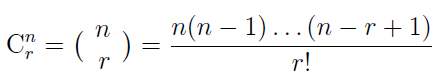
where n ≥ 1 and r ≥ 0 are integers, r ≤ n. Create a function M-file comb.m containing the function comb(n,r):
function y=comb(n,r)
if r = = 0 % no space between the two equal signs
y=1;
return
end
top=prod([n:-1:n-r+1]);
bottom=prod([1:r]);
y=top/bottom;
Now enter after the prompt
comb(4,0) , comb(3,3) , comb(5,2) , comb(9,5) , comb(25,14)
Example 2: Consider the function
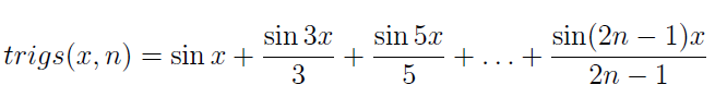
where x is the point (or array of points) where the function is being evaluated and n is the number of terms used in this series of sine functions. For example,
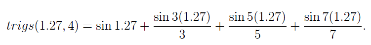
Construct the function M-file trigs.m:
function y=trigs(x,n)
% commence the sum for y with the first term
y=sin(x); % y is an array if x is an array
for k=2:n
kodd=2*k-1;
y=y+sin(kodd*x)/kodd;
end
Now evaluate trigs(1.27, 4) (=0.8347) and trigs(1.27, 40) (=0.7822).
You can, of course, now plot a graph of trigs(x, n) for a given n. Construct the following script M-file and then run it.
clear all
x=linspace(-2*pi,2*pi,801);
y=trigs(x,4);
axis([-2*pi 2*pi -1 1])
hold on
plot(x,y)
hold off
Change the trigs(x,4) to each of trigs(x,40) and trigs(x,200) and execute. The graphs you see are part of Fourier Series theory.
fplot, fzero, fminbnd, quadL
Functions operating on functions: fplot, fzero, fminbnd, quadL
Suppose a function y = func(x) has been defined in a function M-file func.m. Then
- fplot(@func,[a b]) or fplot(’func(x)’,[a b]) plots the function for a ≤ x ≤ b without requiring you to set up arrays
- fzero(@func,[a b]) or fzero(’func(x)’,[a b]) finds a root of the equation func(x) = 0 inside the interval [a, b] providing func(a) and func(b) have opposite signs. fzero(@func,c) or fzero(’func(x)’,c) finds a root of the equation func(x) = 0 by commencing a search at x = c.
- fminbnd(@func,a,b) or fminbnd(’func(x)’,a,b) finds the coordinates of a minimum point for a ≤ x ≤ b.
- quadL(@func,a,b) or quadL(’func(x)’,a,b) finds an accurate value for the integral from a to be of func(x) dx.
Note: quadL uses arrays in its calculations. Hence the M-file func.m must use the array dot notation in the definition of func(x). This is not required for fplot, fzero or fminbnd.
Example: Consider the function f1(x) = x − cos x / 2 + x2 . Define it in the function M-file f1.m.
function y=f1(x)
% use dots as quadL(@f1,a,b) occurs in calling M-file
y=(x-cos(x))./(2+x.^2); % ";" to avoid printing inside f1.m
Now construct and execute the following M-file. This will graph the function for −10 ≤ x ≤ 10, find its zero (from the graph, between 0 and 1), find the x and y coordinates of the minimum and integrate the function from the x-intercept to x = 10.
clear all
fplot(@f1,[-10 10])
hold on
plot([-10 10],[0 0],’k’) % adds x-axis
hold off
x_intercept=fzero(@f1,[0 1])
[xmin,ymin]=fminbnd(@f1,-3,3) % finds both the x-coordinate
% and y-coordinate of minimum
accurate_integral=quadL(@f1,x_intercept,10)
As well as the graph, the following output should result:
x_intercept = 0.7391
xmin = -0.4562
ymin = -0.6132
accurate_integral = 1.8910
Exercise 1: Consider the output OP(t) = 1 − 4e−t sin t for t ≥ 0. Define this function in an M-file and then use fplot to graph it for 0 ≤ t ≤ 5, find the two zeros, find its minimum value and evaluate the integral from 0 to 5 OP(t) dt.
Exercise 2: Knowing that tan x has a vertical asymptote at x = π/2, see what occurs if you enter after the prompt fplot(@tan,[1 2]). Remember that tan x is already stored in tan.m. Knowing that √x only exists for x ≥ 0, see what occurs if you enter fplot(@sqrt,[-1 4]).
7. Polynomials
MATLAB has a number of commands to make manipulating and evaluating polynomials very simple. In the Help Window, in the \mat\polyfun topic you will see the following commands:
roots - Find polynomial roots
poly - Convert roots to polynomial
polyval - Evaluate polynomial
polyvalm - Evaluate polynomial with matrix argument
residue - Partial-fraction expansion (residues)
polyfit - Fit polynomial to data
polyder - Differentiate polynomial
conv - Multiply polynomials
deconv - Divide polynomials
In MATLAB (but not in the “Maple” Symbolic Math Toolbox) a polynomial is represented by an array (row vector) of its coefficients in descending order. For example, enter the polynomial p(x) = 3x5−4x4+7x2 −9x+3 as p=[3 -4 0 7 -9 3].
What polynomial q(x) does q=[4 5 -6] represent?
MATLAB does not provide a special function for adding or subtracting polynomials other than using arrays of the same length. Hence you would need to pad out the shorter array with leading zeros in this circumstance. Note that when poly forms a polynomial with given roots, it makes the leading coefficient equal to one. A few of these concepts are illustrated by executing the following M-file. Examine carefully the output.
clear all % file available in M-files folder as file4.m
p=[3 -4 0 7 -9 3]
q=[4 5 -6], qpadded=[0 0 0 4 5 -6];
newp=p+2*qpadded
proots=roots(p)
qroots=roots(q)
p1=poly(proots) % check that p=3*p1, as expected
q1=poly(qroots) % check that q=4*q1, as expected
y=polyval(p,2.31) % evaluate p(2.31)
pder=polyder(p) % check answer is dp/dx
qder=polyder(q) % check answer is dq/dx=8*x+5
pq=conv(p,q) % multiply p(x)*q(x)
[Q,R]=deconv(p,q) % Q=quotient, R=remainder for p/q
Exercise: Add the commands x=linspace(-1.7,2,300); plot(x,polyval(p,x)) to the previous M-file to see a graph of y = p(x) for −1.7 ≤ x ≤ 2.
8. Symbolic Toolbox
In all previous sections of this introduction MATLAB has been used as a powerful programmable graphics calculator. A variable x must have a numerical value (or array values) before expressions involving x can then be evaluated. For example if you merely enter the single command sin(x) after the prompt you receive the error message
??? Undefined function or variable ’x’.
However, commands in the Symbolic Math Toolbox enable you to enter formulae such as sin(2*x), x*exp(x), x^2+3*atan(x), cos(x)^2+sin(x)^2, etc, where x is a symbolic variable. Each expression can be given a variable name (also symbolic) thereby allowing algebraic, trigonometric and other functional manipulations and simplifications as well as permitting differential and integral calculus. You will be solving and computing with mathematical symbols rather than numbers.
The tools in the Symbolic Math Toolbox are built upon the core of the powerful software program called Maple® which is used in many universities in Australia and overseas. For convenience only in this guide we will refer to the smaller Symbolic Math Toolbox attached to Matlab as “Maple”. The interface between Matlab and “Maple” is smooth and it is easy to move in and out of this Symbolic Math Toolbox.
The simplest way to enter “Maple” is to make one or more variables into symbolic symbol(s) using the syms command. Enter the following and examine the output:
syms x
y=x^2-5/x % y is automatically another symbolic variable
z=y*x-8 % z is automatically another symbolic variable
You notice that no attempt has yet been made to simplify z. Add the command z=simplify(z).
Note that in earlier versions of Matlab the first two lines above were equivalent to the single command y=’x^2-5/x’. This notation for constructing a symbolic expression using single quotation marks is still valid in many parts of “Maple” although it is being phased out because MATLAB already uses single quotation marks in other situations. Often in the “Maple” help menu you will still see the single quotation formulation but it is recommended you ignore it wherever possible to avoid confusion.
Numbers can be held in various possible formats in “Maple”. The default format is an integer or rational fraction. If this is not possible, a real number will be approximated by a fraction of large integers. The sym function converts the argument into a symbolic expression in “Maple”. Conversely, the double function converts a symbolic number back into a double-precision value in MATLAB. In each of the following cases the symbolic expression in the middle column results from the corresponding sym command, while the last column results if you then apply the double(...) command to each symbolic value in the middle column:
| sym(11/13) | 11/13 | 0.8462 |
| sym(3.85) | 77/20 | 3.8500 |
| sym(pi) | pi | 3.1416 |
| sym((4/5)^2) | 16/25 | 0.6400 |
| sym(sqrt(49)) | 7 | 7 |
| sym(sqrt(51)) | sqrt(51) | 7.1414 |
| sym(exp(1)) | 6121026514868073*2^(-51) | 2.7183 |
| sym(sin(1)) | 7579296827247854*2^(-53) | 0.8415 |
Alternative formats can be viewed by entering help sym.
Exercise: What do you expect to result if you enter the following?
syms x
y=x+1.4*sqrt(x+3)+5.49
pretty(y) % output to look like type-set mathematics
Algebraic operations
A selection of commands in “Maple”:
| simplify | performs algebraic and other functional simplifications |
| simple | tries a number of simplification techniques including trigonometric identities; may need using twice |
| collect | collects like terms |
| factor | attempts to factor the expression |
| expand | expands all terms |
| poly2sym | converts array of polynomial coefficients in \mat into a symbolic expression in ‘‘Maple" with x as the variable |
| sym2poly | converts symbolic polynomial in ‘‘Maple" into coefficient array in MATLAB |
At the simplest level, enter factor(28809).
Example 1: Suppose p(x) = x2(x + 4)2 − 8x(x + 1)2 + 13x − 6. Expand and factor in “Maple”, convert into an equivalent Matlab array, find the roots numerically, re-assemble the polynomial coefficients from the roots and then change back into a symbolic form.
clear all % file available in M-files folder as file5.m
syms x
p=x^2*(x+4)^2-8*x*(x+1)^2+13*x-6;
p=expand(p)
p=factor(p)
P=sym2poly(p) % change into MATLAB array P
polyroots=roots(P) % numerically find roots in \mat
Q=poly(polyroots) % re-assemble polynomial from its roots
q=poly2sym(Q) % change back to Maple expression
You will notice that the coefficients of x3 and x2 in q(x) are not exactly zero but are infinitesimally small due to tiny round-off errors introduced when numerically solving for the roots in MATLAB.
Example 2: Using trigonometric identities you should be able to show that
sin x/cos x − sin x + sin x/ cos x + sinx is equivalent to tan 2x.
Use simple in “Maple” to check this.
clear all % file available in M-files folder as file6.m
syms x
y=sin(x)/(cos(x)-sin(x))+sin(x)/(cos(x)+sin(x));
pretty(y)
y=simple(y)
Solving
You have seen that fzero numerically finds where a function is zero in MATLAB. “Maple” uses the solve facility which can solve n simultaneous algebraic or transcendental equations for n unknowns. It firstly attempts to find an exact analytic solution. If this is not possible, it then attempts to find a numeric solution in variable precision format.
The command is of the form [a1,a2,...,an]=solve(f1,f2,...,fn,v1,v2,...,vn).
Here, f1,f2,...,fn are symbolic expressions that are to be made zero, v1,v2,...,vn are the variables in alphabetical order to be solved for, and a1,a2,...,an are the corresponding answers.
Solving a single equation
To solve a single equation f(x) = 0, this reduces to a=solve(f,x).
Of course there might be more than one solution for a. What happens if you do not specify the variable for which the equation is to be solved? If there is only one symbolic variable in the expression, it will solve for it by default. Otherwise x is the default variable. If there are two or more symbolic variables, none of which is x, and you forget to specify the one for which the solution is required, it appears to choose the last alphabetical one.
Example 1: Solve the equation
10/x2 + 1 = 4− x. This is equivalent to solving 10/x2 + 1 − 4 + x = 0. There are various ways:
clear all
syms x
f=10/(x^2+1)-4+x; % f is now a symbolic expression
soln=solve(f,x) % note the three solutions
or, knowing that x is the default variable,
clear all
syms x
soln=solve(10/(x^2+1)-4+x) % no need to use f or specify x
In earlier versions of MATLAB, you could use
clear all
soln=solve(’10/(x^2+1)=4-x’)
but this is being phased out.
Exercise: Change to 10/(x^2+1)+2+x=0 and solve again.
Example 2: Solve the general quadratic equation ax2 + bx + c = 0 for x.
clear all
syms a b c x
soln=solve(a*x^2+b*x+c)
giving the output soln=[1/2/a*(-b+(b^2-4*a*c)^(1/2))]
[1/2/a*(-b-(b^2-4*a*c)^(1/2))]
However, if for some reason you wanted to solve the same equation for b, you would need
clear all
syms a b c x
soln=solve(a*x^2+b*x+c,b)
giving the ouput soln=-(a*x^2+c)/x.
Example 3: We know sin θ = 0.5 has an infinite number of solutions. Enter
clear all
syms theta
angle=solve(sin(theta)-0.5)
giving the output angle=1/6*pi.
Example 4: Unlike Example 3, the equation sin θ = 0.5 − cos θ, −π ≤ θ ≤ π, does not have obvious solutions. But “Maple” can find two solutions exactly. The answers are hardly in a form that you would use and so it is better to convert them into numeric values.
clear all
syms theta
angle=solve(sin(theta)-0.5+cos(theta)) % hardly usable
angle=double(angle) % looks better in MATLAB
giving the output angle=[atan((1/4-1/4*7^(1/2))/(1/4+1/4*7^(1/2)))]
[atan((1/4+1/4*7^(1/2))/(1/4-1/4*7^(1/2)))+pi]
angle=-0.4240
1.9948
Example 5: By means of a simple sketch you can see that ex = 4− x2 has two solutions.
However, there is no analytic way to find them. Enter
clear all
syms x
soln=solve(exp(x)-4+x^2)
giving the output soln=1.0580064010906363086213874461232. This indicates that a numerical solution process was needed in “Maple”, and the answer is in variable precision format. If you wish, you can follow with soln=double(soln). Note that only the solution nearest to zero was found.
Solving simultaneous equations
Find the points of intersection of the two circles 2x2 − x + 2y2 − 8y = 0 and x2 + 2x + y2 − 6y + 1 = 0.
clear all % file available in M-files folder as file7.m
syms x y
eqn1=2*x^2-x+2*y^2-8*y;
eqn2=x^2+2*x+y^2-6*y+1;
[X,Y]=solve(eqn1,eqn2)
giving the output X = [ 2] Y = [ 3]
[ -14/41] [ 3/41]
which implies the two points (x, y) = (2, 3) and (x, y) = (−14/41, 3/41).
subs, eval
Variable substitution and expression evaluation: subs, eval
Suppose you have a symbolic expression f which includes the symbol x and you wish to substitute for x another symbol c or a numerical value x0. Then you can use the general subs command g=subs(f,old,new) which in our cases would be g=subs(f,x,c) or g=subs(f,x,x0). Here old, new can be arrays. The result g is still a symbolic variable or symbolic constant in “Maple”.
Example 1: Consider a function of the two Cartesian coordinates f(x, y) =
2xy/(x2 + y2)2 .
Change to polar coordinates using x = r cos θ, y = r sin θ and then determine the value of f at an arbitrary point on the unit circle r = 1.
clear all
syms x y r theta
f=2*x*y/(x^2+y^2)^2;
F=subs(f,[x y],[r*cos(theta) r*sin(theta)]);
F=simple(F) % previous answer is messy
f_on_unit_circle=subs(F,r,1)
which gives the output
F=sin(2*theta)/r^2
f_on_unit_circle=sin(2*theta)
An alternative is to use the eval command. It is of the form ans=eval(S) where S is a symbolic expression for which at least one of its symbolic variables has just been given a value. If all variables are given numerical values, the answer is a number in MATLAB, not “Maple”.
Example 2: Let us compare simple MATLAB and “Maple” codes which both evaluate the expression y = (x3 + 2) sec x at x = 0.123.
| MATLAB code | Maple code using subs | Maple code using eval |
| clear all | clear all | clear all |
| x=0.123 | syms x | syms x |
| y=(x^3+2)*sec(x) | S=(x^3+2)*sec(x); | S=(x^3+2)*sec(x); |
| y=subs(S,x,0.123) | x=0.123; | |
| y=double(y) | y=eval(S) |
Example 3: Reconsider Example 1 at the top of the page. Change the last line to the corresponding two lines in the following M-file:
clear all
syms x y r theta
f=2*x*y/(x^2+y^2)^2;
F=subs(f,[x y],[r*cos(theta) r*sin(theta)]);
F=simple(F)
r=1;
f_on_unit_circle=eval(F)
ezplot
If S is s symbolic expression, then ezplot(S,[a b]) graphs the function y = S(x) (or y = S(t)) over the domain a ≤ x ≤ b. If [a b] is omitted, the default domain is −2π ≤ x ≤ 2π. Also, if no title command is used, the default title is the expression S. Of course you are not using arrays and so the dot notation is not applicable.
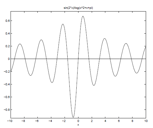
Example: In “Maple”, plot the function y = sin 2x/ ln(x2 + x + π) for −10 ≤ x ≤ 10.
clear all % file available in M-files folder as file8.m
syms x
y=sin(2*x)/log(x^2+x+pi);
ezplot(y,[-10 10]) % notice title
hold on
plot([-10 10],[0 0],’k’) % plot x-axis
hold off
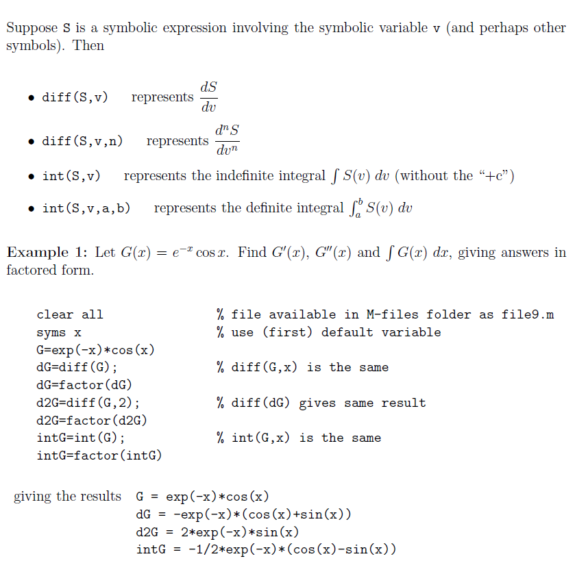
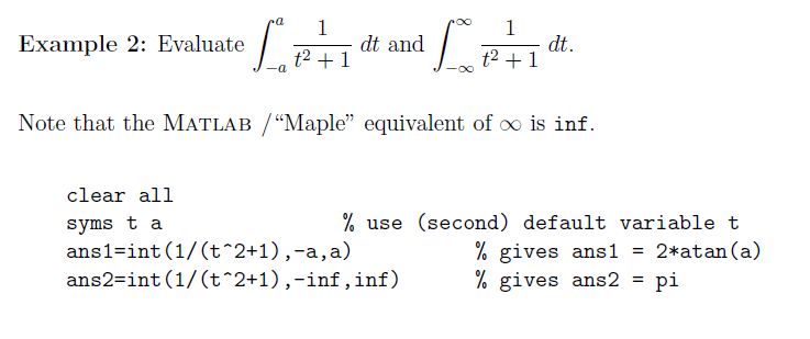
diff and int
Although there are many other calculus commands that will be needed later, we will restrict the discussion to diff and int in this introduction.
The default variable is x; otherwise it is t; but if you wish to differentiate or integrate with respect to some other symbol, say v, it must be specified.
9. Matrices and Vectors
Each array that was discussed in Section 4 was, in effect, a row vector or row matrix. But you are aware that a rectangular array represents a matrix and a single array column represents a column vector.
To construct a matrix with m rows and n columns (called an “m by n matrix”, written m×n matrix), each row in the array ends with a semicolon. For example, run the following M-file mat.m:
A=[3 -5 1;-2 0 -4;6 7 9]
B=rand(3,3)
C=[1 -3;-1 5;2 8]
The element A(i,j) is in the ith row and jth column. Hence, after the prompt, enter
a23=A(2,3), b31=B(3,1), c12=C(1,2)
The comma separates the row number(s) from the column number(s).
What is A(3,[2 3]), B([1:2:3],[1:2:3])?
A single colon “:” before the comma means “take all rows”, whereas a single colon after the comma means “take all columns”. Hence A(:,2) is column number 2 in the matrix A while ![]() is the first row of B.
is the first row of B.
Providing matrices have the same shape they can be added or subtracted. Providing they have compatible shapes they can be multiplied using the established rules for matrix multiplication. Hence calculate after the prompt D=2*A-B, F=A*B, G=A*C, Asq=A^2. However, B+C and C*A produce error messages.
Note: A.^2 does not square the matrix but squares each element in the matrix. Similarly, A.*B is not matrix multiplication but merely multiplies the corresponding positions in the two matrices.
det(A) is the determinant of A, written |A|.
A' is the transpose of A and is written in mathematics as AT. It is formed by interchanging the rows and columns. Hence, if you need to input the column vector
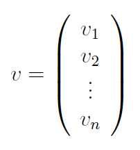
you could enter v=[v1;v2;...;vn] or v=[v1 v2 ...vn]'.
The magnitude or Euclidean norm of the vector v, given by
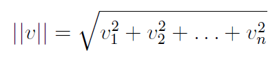
is represented in MATLAB by norm(v).
If A is a square matrix with |A| = 0, then inv(A) represents the inverse of A, denoted in mathematics by A−1.
The n × n identity matrix I is represented in MATLAB by eye(n). For the matrix A at the beginning of this section, verify that A*inv(A)=inv(A)*A=eye(3).
10. Other Commands
Previous students have found other commands useful and have suggested they be included in this introduction. Also included are examples that further illustrate efficient usages of commands already discussed.
global
Often a variable (which could be a scalar variable, or an array, or a symbolic variable representing a mathematical expression) has been determined in one M-file and might also be needed in another M-file, for example a function M-file. However, it might not be practical or possible to pass it across as an input variable to the function. Two M-files can share a common Matlab workspace for a variable var if the command
global var
occurs in both M-files before it is defined or used in either.
limits
Suppose you need to find the limit ie,

for which both the numerator and denominator tend to zero. This is an example of an indeterminate form of which many others will be investigated in later mathematics using L’Hôpital’s Rule. One method is to find the limit graphically. Enter:
clear all
syms x
f=(2^x-2)/(2*x-2);
ezplot(f,0.95,1.05)
zoom on
You might notice a small hole in the graph at  because the expression is undefined there. However, by zooming in, you see that the function is tending towards a value 0.6931 as x → 1. Do you recognise this value? To obtain an exact answer, use the “Maple”s limit command. Add to the above M-file the extra command lim=limit(f,x,1) to obtain the answer lim = log(2) (which is ln 2).
Exercise 1: Change the previous M-file to demonstrate that

both graphically and using limit.
Exercise 2: Change the previous M-file to find
^{tan 2 \pi x}")
(clearly undefined at x = 0.25)
to obtain 0.3679 graphically and 1/e using limit.
funtool
The command funtool opens an interactive graphical function calculator that uses mouse clicks to perform operations on symbolic expressions. It can simultaneously manipulate and graph (in two separate windows) two functions ") and
and ") and allows constant horizontal shifts. A third window controls the calculator, and contains the symbolic functions f and g, the chosen domain of these functions, and a constant value a.
and allows constant horizontal shifts. A third window controls the calculator, and contains the symbolic functions f and g, the chosen domain of these functions, and a constant value a.
Below this are four rows of buttons that enable you to combine and operate on f and g in a variety of ways as well as controls for the calculator itself.
Try funtool when you have some time to help visualise how functions behave and interact.
diff command
You should have discovered that the diff command has a different meaning in MATLAB compared to “Maple”. In MATLAB diff(vec) finds the differences between elements in the array vec. In “Maple”, if S is a symbolic expression, diff(S) finds its derivative.
However, you know that
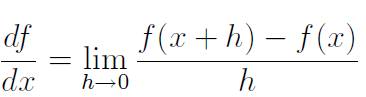
Hence, if the differences are divided by a tiny step-size they should be crude approximations to the derivative.
maximum
You are aware that the MATLAB commands max, min find the maximum and minimum elements in an array (and their locations) while fminbnd helps to find the minimum value of a function defined in a function M-file. Seeing there is no such command as fmaxbnd, how can we print out the maximum value of a function f(x), for a ≤ x ≤ b, without using the zoom on facility? For example, find the x and y coordinates of the maximum turning point of y = xe−x cos x, 0 ≤ x ≤ π.
Using MATLAB
The value of x where f(x) has a maximum is the same as the value where −f(x) is a minimum. Hence, set up the function M-file negf.m
function y=negf(x)
y= - x*exp(-x)*cos(x);
and run the following M-file
clear all
[temp1,temp2]=fminbnd(@negf,0,pi);
xmax=temp1, ymax= -temp2 % gives xmax=0.5959, ymax=0.2718
Using “Maple”
Solve for where the derivative is zero and then substitute back into y = f(x). However, be aware that there might be other (real or complex) solutions to the equation df/dx = 0.
clear all
syms x
f=x*exp(-x)*cos(x);
xmax=double(solve(diff(f))) % gives xmax=0.5959
x=xmax;
ymax=eval(f) % gives ymax=0.2718
11. Troubleshooting
In previous years students have experienced various problems. We have collected some "frequently asked questions” with answers in the hope it will save you some time.
Question:
I tried to execute my M-file proj.m using >> proj but received
??? Undefined function or variable ’proj’.
or
I tried to use my function proj(x) held in proj.m but received
??? Can not find function ’proj’.
Error in ==> c:\\mat\toolbox\\mat\specgraph\fplot.m
On line 85 ==> x = xmin; y = feval(fun,x);
Reason:
You are not working in the same directory where the M-file proj.m is held.
Action:
Change directory or save the M-file into the correct directory .
******************************************************************************
Question:
I attempted to evaluate an elementary MATLAB function such as mod(101,7) (or another MATLAB function) but received the following message
??? ??? Error using ==> mod
Too many input arguments.
I then asked for help using help mod and received
No help comments found in mod.m.
Reason:
Both responses indicate that you have inadvertently named one of your own M-files mod.m previously. It has taken precedence over MATLAB ’s inbuilt function.
Action:
Change the name of your own M-file to one that does not exist in MATLAB .
******************************************************************************
Question:
Why do I receive one of the following error messages, or similar?
??? Error using ==> .*
Matrix dimensions must agree.
or
??? Error using ==> plot
Vectors must be the same lengths.
Reason:
When doing a calculation involving two arrays, or graphing using the plot command, the arrays must be of the same size.
Action:
Check the size of each array involved.
******************************************************************************
Question:
Why did I not get any numbers printed on the screen?
Reason:
Semicolons at the end of a MATLAB assignment statement prevent answers being displayed.
Action:
Leave off semicolons where you want numbers to be shown in the output.
******************************************************************************
Question:
Why did I get thousands of numbers printed on the screen?
Reason:
Semicolons at the end of a MATLAB assignment statement prevent answers
being displayed.
Action:
Place semicolons where you do not want numbers to be shown in the output.
******************************************************************************
Question:
Why do I continually get the following error message?
??? Error using ==> ^
Matrix must be square.
or
??? Error using ==> *
Inner matrix dimensions must agree.
Reason:
You have asked for something like x^2 or f(x)*g(x) where x is currently an array. It is only possible to square an array x or multiply f(x)*g(x) if x is a square matrix.
Action:
If you think x is a scalar variable, it is possible that you were also using the same symbol to represent an array and forgot to clear it. But more likely x is an array and you should be using the dot notation x.^2 or f(x).*g(x). The location might be in a script M-file or, more obscurely, in a function M-file where you did not allow for later array evaluations.
******************************************************************************
Question:
Why are parts of my graphical figures missing?
Reason:
You have probably lost graphs or graphical components.
Action:
Make sure each figure is numbered. Within a figure, use the hold on . . . hold off facility to avoid losing command outcomes.
******************************************************************************
Question:
When I access a function M-file, either by doing an evaluation after the >> prompt or else calling from another M-file, why do I get no answer back or else receive the empty answer: [ ] ?
Reason:
Although the first line in your function M-file was of the form
function y=fred(x)
you have not assigned any value to y during the file.
Action:
Make sure output variables are given values in function M-files.
******************************************************************************
Question:
When using solve on a transcendental equation in “Maple”, why do I get complex solutions, or else a real solution which is not the one I want?
Reason: Consider, for example, the equation xex + x3 −2 = 0. Using
syms x , ans=solve(x*exp(x)+x^3-2)
yields a complex solution only.
Action:
Use fzero in MATLAB instead. If the function has been defined in func.m, then ans=fzero(@func,[0 1]) yields ans=0.7482 which is probably the solution you were seeking within the specified interval.