Introduction to Stata
| Site: | learnonline |
| Course: | Research Methodologies and Statistics |
| Book: | Introduction to Stata |
| Printed by: | Guest user |
| Date: | Tuesday, 26 May 2026, 7:40 AM |
1. What is Stata?
![]() According to StataCorp (2016), Stata is “a complete, integrated statistical software package that provides everything you need for data analysis, data management, and graphics”. Basically, Stata is a software that allows you to store and manage data (large and small data sets), undertake statistical analysis on your data, and create some really nice graphs.
According to StataCorp (2016), Stata is “a complete, integrated statistical software package that provides everything you need for data analysis, data management, and graphics”. Basically, Stata is a software that allows you to store and manage data (large and small data sets), undertake statistical analysis on your data, and create some really nice graphs.
This software is commonly used among health researchers, particularly those working with very large data sets, because it is a powerful software that allows you to do almost anything you like with your data.
It’s important to note that Stata is not the only statistical software – there are many others that you may come across if you pursue a career that requires you to work with data. Some of the other common statistical packages include SPSS and SAS (yes, they all start with ‘s’!). The focus for this session, however, is on Stata.
![]() Task: Open the Stata program
Task: Open the Stata program
Open the Stata program by clicking: Start menu > All Programs > Stata 14 > StataIC 14
2. Navigating the Stata interface
![]() When you first open Stata on your computer, you should see a window that looks similar to this:
When you first open Stata on your computer, you should see a window that looks similar to this:
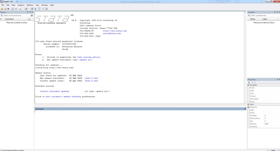
The Stata user interface is made up of several ‘windows’: 1) Review; 2) Results; 3) Command; 4) Variables; and 5) Properties. All these windows (except the Results window), has its name it its title bar.
Review
The Review window keeps a record of all commands Stata has run, both successful and unsuccessful. This can help you keep track of what you have done. You can copy and paste commands to this window, and can also re-run commands from this window.
Results
This window shows you the results of what you have commanded Stata to do. Even when you just open a file, it will give you a ‘result’ in this window. The Results window is especially useful for finding out when something has not worked, or that it’s actually gone wrong. For instance, if you think you told Stata to create a new variable, the results window will tell you whether or not you actually did create a new variable.
Command
Here is where you enter the commands (words that Stata recognises and associates with a specific task) to tell Stata what you’d like to do with your data.
Variables
This window gives you a neat summary of all the variables in your current dataset, and also includes information about the variables (their properties).
Properties
The Properties window displays various variable and dataset properties. This window is particularly useful when you are using one or a set of variables, as it displays properties that are shared across those particular variables. You can also change variable and dataset properties using the Properties window.
3. Defining the working folder
![]() Before doing anything with an open Stata file, you should always define the location of your working folder. Your ‘working folder’ is a folder on (one of) your drives where you keep all of your data for a particular project or piece of analysis.
Before doing anything with an open Stata file, you should always define the location of your working folder. Your ‘working folder’ is a folder on (one of) your drives where you keep all of your data for a particular project or piece of analysis.
If you have never been so organised with your data sets, now is an excellent time to start! There’s really not a whole lot worse than doing a bunch of analyses using multiple datasets and having the files all jumbled in with other documents … or worse, spread all over the place in separate folders!
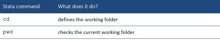
There are two key commands for defining and checking your working folder:
We are now going to define our own working folder, which will be our USB drive location. Now would be a perfect time to get out your USB stick, plug it in, and then open windows explorer to determine the file path for your USB.
![]() Task: Define and check your working folder
Task: Define and check your working folder
Make sure you know where you’d like to keep the data files (and other related documents) for this workshop. You might choose to create a new folder on your USB drive for this purpose (this would be our strong recommendation!).
Use the cd command to define your working folder location, e.g.,:
. cd "E:\Stata_workshop"
You can then check the current working folder using the pwd command:
. pwd
4. Opening data
![]() It may come as a surprise to you that we are covering something as basic as opening a data file in this session. However, when we use software like Stata, we move away from clicking through menus to tell the program what we want it to do. So we need to learn some basic commands to even just open our data file so that we can do something with the data.
It may come as a surprise to you that we are covering something as basic as opening a data file in this session. However, when we use software like Stata, we move away from clicking through menus to tell the program what we want it to do. So we need to learn some basic commands to even just open our data file so that we can do something with the data.
Here are some of the key commands we can use to open data in Stata:
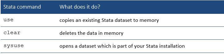
Normally we would have a data set (or seven, or fifty two!) that we want to open and do something with. If we have this data set saved (in Stata format!) and stored in our working folders, we could access it using the following use command:
. use “filepath\filename.dta”, clear
If you had a Stata data file called “toothbrushes.dta” saved in your C:\ drive, your use command would look like this:
. use “C:\toothbrushes.dta”, clear
It’s good practice to use the clear command after the use command, just in case you already had a dataset open and you’d forgotten … this could lead to you doing things to your other data set that you did not want to do, such as renaming variables, creating new ones, or even worse … deleting variables or data!
Now we’re going to actually open a data set … we know, this is exciting! We’re going to open and use a dataset that comes with the Stata software package, with data on life expectancy from different countries around the world. This data set is called “lifeexp.dta” and is stored in the same location as your Stata software. We don’t need the file path and file extension (.dta) included in our command (like we did with the use command), because the sysuse command tells Stata that it’s using its own data file.
![]() Task: Open a Stata demonstration data file
Task: Open a Stata demonstration data file
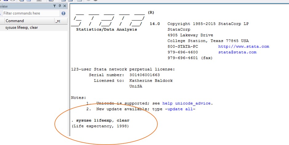
Type the following command into your command window:
. sysuse lifeexp, clear
Have a quick look at your results window … what can you see? Probably it doesn’t seem like much … you should (hopefully) get something like this:
5. Looking at your data
![]() Sometimes when you open a data set you just want to have a look at it. You can do this by going to Data > Data Editor > Data Editor (Browse) from the menus, or by typing the command browse.
Sometimes when you open a data set you just want to have a look at it. You can do this by going to Data > Data Editor > Data Editor (Browse) from the menus, or by typing the command browse.
![]() Task: Browse (have a look at) a data file
Task: Browse (have a look at) a data file
Type the following command into your command window:
. browse
This command will open the current data file in use, so no need to specify the file name after the command. Typing in this command should open a new data editor window with the life expectancy data, like this:
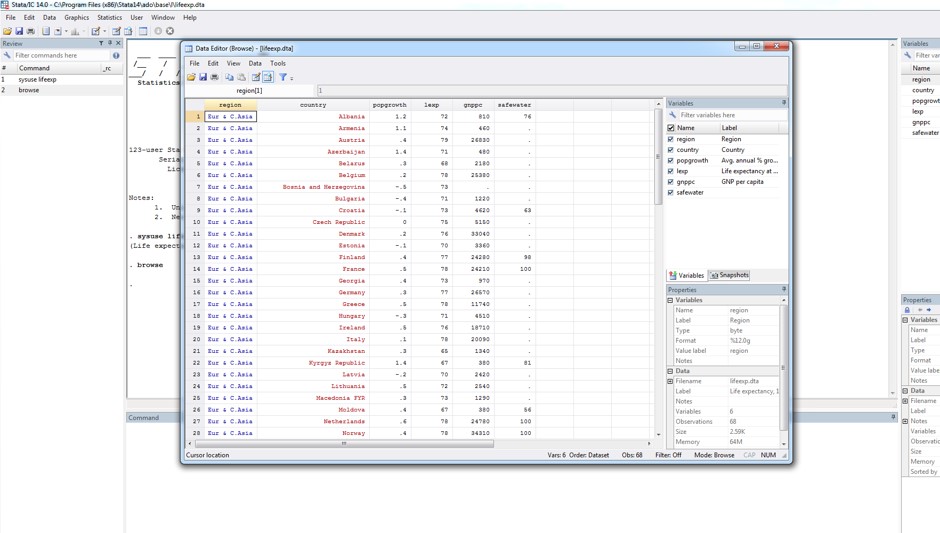
The data editor window is the window that opens on top of the main Stata interface, and looks just like any other ordinary spreadsheet (e.g., MS Excel). You can see the variable names along the top of the columns, the case numbers down the left hand side, and the actual data in each of the cells.
6. Saving data
![]() Obviously when you create or are given a data set for your work, you need to save this file somewhere sensible. It’s really bad practice to use it from your ‘downloads’ folder, or your desktop (just for example … and yes, people actually do this … but not you!).
Obviously when you create or are given a data set for your work, you need to save this file somewhere sensible. It’s really bad practice to use it from your ‘downloads’ folder, or your desktop (just for example … and yes, people actually do this … but not you!).
There are two key commands for saving and replacing a data file:
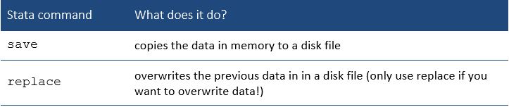
So, once you’ve decided where you’re going to save your files (you would have already done this when defining your working folder, so we should be ok at this point), you can use the save command to save your file where you want it, e.g.,:
. save " E:\Stata_workshop\lifeexp_revised.dta"
You can add the replace command after a comma at the end of the save command if you already have a data set in the same location by the same name and you wish to replace it.
. save "E:\Stata_workshop\lifeexp.dta", replace
If you do not wish to replace the file, you’ll need to save the data set under a new name, as per the first save example.
![]() Task: Save your data set
Task: Save your data set
Save your data set to your working folder for this workshop (on your USB drive, where your working folder is), e.g.:
. save " E:\Stata_workshop\lifeexp.dta"
7. Basic data description
![]() Before you can start doing data analyses, you need to familiarise yourself with the data. I like to call this ‘getting to know your data’. There are several commands that help you to understand the characteristics your data. Some of these commands provide similar information and it’s up to you which ones you prefer to use. However, before initiating data analyses, remember to always check the frequencies of all variables, how categorical variables have been coded, the minimum and maximum values and number of missing observations. This is a good way to identify any outliers and potential mistakes in the dataset.
Before you can start doing data analyses, you need to familiarise yourself with the data. I like to call this ‘getting to know your data’. There are several commands that help you to understand the characteristics your data. Some of these commands provide similar information and it’s up to you which ones you prefer to use. However, before initiating data analyses, remember to always check the frequencies of all variables, how categorical variables have been coded, the minimum and maximum values and number of missing observations. This is a good way to identify any outliers and potential mistakes in the dataset.
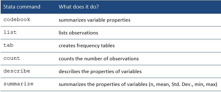
There are several commands for describing your data:
![]() Task: Get to know your data set
Task: Get to know your data set
Try typing some of the data description commands:
. count
. describe
. summarize
. codebook
. list
If you want to check the frequencies for a certain variable, type e.g.:
. tab region
If you want to also include the missing values, type e.g.:
. tab region, missing
You can combine the data description commands with qualifiers and operators. For example, if is a qualifier which is used to select the observations to which a command applies. Operators used in Stata can be found in the Table below:
Operators in logical expressions:
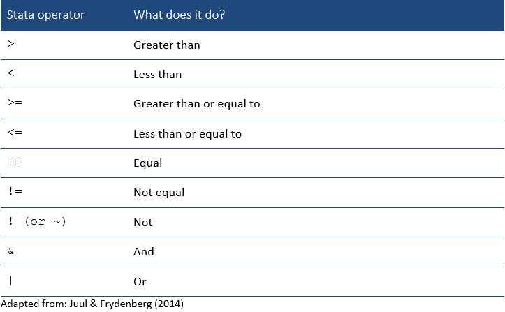
If you want to list countries with missing information for the variable gnppc (GNP per capita) , type e.g.:
. list country gnppc if gnppc==.
If you want to list countries with life expectancy less than 65 years, type e.g.:
. list country lexp if lexp <65
8. Basic variable recoding
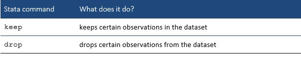
![]() In this intro, we’re not going to cover a lot of data manipulation. This could include things like checking your dataset for duplicate cases and deleting duplicates. You may also want to analyse only a subset of the study sample. Drop and keep commands can be used to drop/keep certain observations. Remember that once you’ve dropped something, you can’t get it back anymore! Therefore, when saving the revised dataset, use a different file name.
In this intro, we’re not going to cover a lot of data manipulation. This could include things like checking your dataset for duplicate cases and deleting duplicates. You may also want to analyse only a subset of the study sample. Drop and keep commands can be used to drop/keep certain observations. Remember that once you’ve dropped something, you can’t get it back anymore! Therefore, when saving the revised dataset, use a different file name.
There are two key commands analysing subsamples:
If you want to analyse only a subset of dataset, which includes countries with life expectancy 65 years or more, type:
. drop if lexp <65
or
. keep if lexp >=65
Variable recoding is something that everyone will need to do at some point in time. It is usually recommended to create a new variable and not to overwrite the existing one. You may also want to do other modifications to your variables, such as logarithm modifications. After creating new variables, it’s a good practice to label variables and variable values, so that you won’t forget how the recoding was done.
In order to create a new variable called loggnppc which is a logarithm of the values of variable gnppc, type:
. generate loggnppc = log(gnppc)
In order to recode the variable region so that Europe and Asia are coded in the same category and to generate a new variable called region2, type:
. recode region (1=1) (2/3=2), generate(region2)
In order to label the values of variable region2, type:
. label define region2_label 1 "Europe/Asia" 2 "America"
. label values region2 region2_label
![]() Task: Variable recoding
Task: Variable recoding
Try using some of the commands introduced in this section.
9. Using do and log files
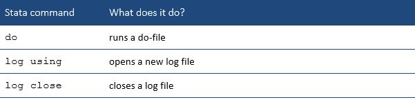
![]() All Stata analyses should be done using do-files. A do-file is a series of commands to be executed in the correct sequence. Do-files document what you did and they are also a good way to identify and correct any mistakes that have been made. Log-files are Stata output files. They also include the documentation of what you did and also your results. A new do-file starts with opening a log file and ends with closing the log.
All Stata analyses should be done using do-files. A do-file is a series of commands to be executed in the correct sequence. Do-files document what you did and they are also a good way to identify and correct any mistakes that have been made. Log-files are Stata output files. They also include the documentation of what you did and also your results. A new do-file starts with opening a log file and ends with closing the log.
There are two key commands for using do and log files:
Example of a Do-file:
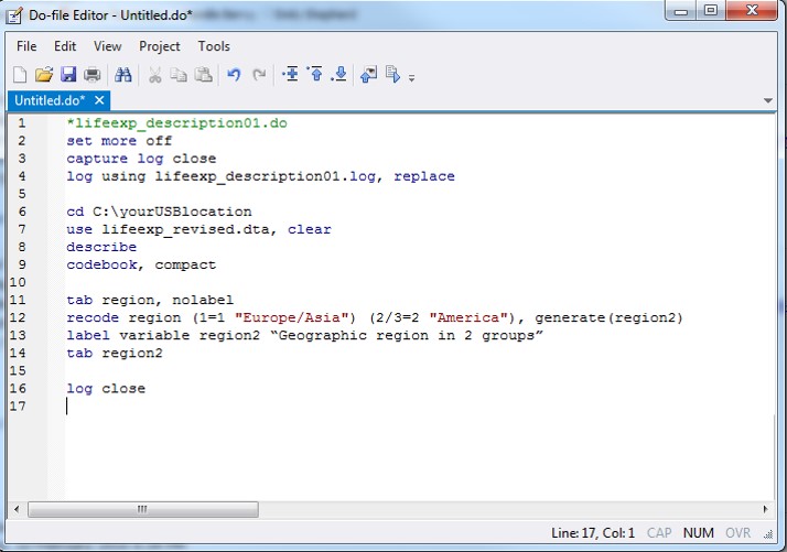
You can add comments to your do-file using and asterisk (*) in front of the comment text, as in the example above.
![]() Task: Do and log files
Task: Do and log files
Insert all your commands to a do-file (such as the example above), run it and inspect (look at) the log file.
10. Getting help
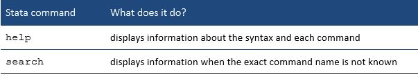
![]() Stata has well-developed help facilities. In addition, Google is always a good way to find help! There are two main commands for getting help in Stata. Depending on whether you know the name of the command, you can use either help or search commands.
Stata has well-developed help facilities. In addition, Google is always a good way to find help! There are two main commands for getting help in Stata. Depending on whether you know the name of the command, you can use either help or search commands.
There are two key commands for getting help:
If you want more information about the tab command, type:
. help tab
If you want more information about duplicates, type:
. search duplicates
Also see the online document 'Stata Manual: Getting Started with Stata for Windows', which is a good introductory manual for Stata:
http://www.stata.com/bookstore/getting-started-windows/
11. References and resources
![]() Juul S & Frydenberg M 2014, An Introduction to Stata for Health Researchers, 4th edn, StataCorp LP, College Station, Texas.
Juul S & Frydenberg M 2014, An Introduction to Stata for Health Researchers, 4th edn, StataCorp LP, College Station, Texas.
Rodriguez, G 2016, Stata tutorial, Princeton University, viewed 23 February 2016, <http://data.princeton.edu/stata/default.html>
Social Science Computing Cooperative (SSCC) 2016, Stata for Researchers: Introduction, SSSC, viewed 23 February 2016, <http://www.ssc.wisc.edu/sscc/pubs/sfr-intro.htm>
StataCorp 2014, NetCourse 101: Introduction to Stata, StataCorp. Information about the course available from: http://www.stata.com/netcourse/intro-nc101/
StataCorp 2016, Stata: data analysis and statistical software, StataCorp, viewed 23 Feruary 2016, <http://www.stata.com/>