Probability and distributions
| Site: | learnonline |
| Course: | Research Methodologies and Statistics |
| Book: | Probability and distributions |
| Printed by: | Guest user |
| Date: | Friday, 8 May 2026, 9:46 PM |
1. Notions of probability
Experiments and Events
Definitions:
- An experiment is a process that leads to a single outcome that cannot be predicted with certainty. The set of all possible results of an experiment is called the support of the experiment (usually called, Omega, W).
- A simple event is an outcome of an experiment that cannot be decomposed into single outcomes. An event is a collection of one or more simple events of interest. Events are generally symbolized by upper case letters, A, B, …., etc.
- Two events are mutually exclusive if they cannot occur at the same time.
Two events are independent events if the occurrence of one does not affect the occurrence of the other.
Examples of experiments:
- Toss a coin once and observe the up face;
- There are two possible results: Head (H), Tail (T);
- W = {H, T}; Simple events:
- Gender of a baby before the normal conception (single baby);
- There are two possible results: male (M), female (F);
- W = {M, F}; Simple events:
- Toss a dice once and observe the up face;
- There are 6 possible results: : 1, 2, …., 6;
- W = {1, 2, 3, , 6}; Simple events:
- The result of tossing a dice is greater than 2: E = {3, 4, 5, 6}.
Probability
Definitions:
- The probability of an event E, P(E): percentage of chances that event E be realized.
- Suppose that an experiment is repeated a large number of times. Each repetition is called a trial. Suppose that for each trial, there is a certain event of interest, E. Then,
- Suppose that an experiment is repeated a large number of times. Each repetition is called a trial. Suppose that for each trial, there is a certain event of interest, E. Then,
P(E) is in fact a relative frequency, as seen in descriptive statistics.
2. Probability distributions
Example: Consider the following gambling experiment which consists in tossing a piece of coin three times. At each toss, the probability of getting Head is equal to, let say p, the player gains $1 if the face up is Head and loses $1 if the face up is Tail. Consider the variable X, the amount of money gained. Then,
|
Sample space |
x = money gained |
P(X = x): Probability that the variable X takes the value x |
|
H H H H H T H T H T H H H T T T H T T T H T T T |
3 1 1 1 -1 -1 -1 -3 |
P(X = 3) = p3 P(X = 1) = p2 (1- p) P(X = 1) = p2 (1- p) P(X = 1) = p2 (1- p) P(X = -1) = p (1- p)2 P(X = -1) = p (1- p)2 P(X = -1) = p (1- p)2 P(X = -3) = (1- p)3 |
The variable X is an example of a discrete variable and its probability distribution:
|
Values x |
P(X = x) |
P(X = x) for p = 0.5 |
|
3 1 -1 -3 |
p 3 3 p 2 (1- p) 3 p (1- p)2 (1- p)3 |
0.125 0.375 0.375 0.125 |
Definition:
- A probability distribution is a mathematical relationship (rule or model) that assigns to any possible value x of a discrete variable X, the probability P(X = x). This rule is also called probability mass function.
The probability for any particular value is between 0 and 1, that is, 0 ≤ P(X = x) ≤ 1, and the sum of the probabilities of all values must be 1, that is, ∑ P(X = x) = 1.
Example:
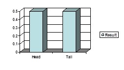
Experiment of tossing a coin once:
- X=observed result.
- Possible outcomes: {H,T}
- P(X = H) =1/2 and P(X = T) = 1/2
Can be summarized: tables, graphs, formulas
Remark: A frequency distribution, discussed in the context of descriptive statistics, can be considered as a sample analogue to the probability distribution. The appropriateness of the model can be validated by comparing the observed sample frequency distribution to the probability distribution (goodness-of-fit test).
3. Probability models used for discrete variables
Example: Consider an experiment in which three (3) white blood cells are tested for lymphocytes. Let L denote a lymphocyte and N denotes a normal cell. Let the probability that a cell is a lymphocyte be 2/3. Then the sample space and corresponding probabilities are:
L L L (2/3)3
L L N (2/3)2 (1/3)
L N L (2/3)2 (1/3)
N L L (2/3)2 (1/3)
L N N (1/3)2 (2/3)
N L N (1/3)2 (2/3)
N N L (1/3)2 (2/3)
N N N (1/3)3
Let the variable X be the number of lymphocytes in the three white blood cells. What is the probability distribution of X?
|
Values of X |
Outcomes |
Probabilities |
|
X = 0 X = 1 X = 2 X = 3 |
N N N L N N or N N L or N L N L L N or L N L or N L L L L L |
P(X = 0) = (1/3)3 = 0.03704 P(X = 1) = 3 (1/3)2 (2/3) = 0.22222 P(X = 2) = 3 (2/3)2 (1/3) = 0.44444 P(X = 3) = (2/3)3 = 0.29630 |
|
|
|
The expected value (average value) of a discrete random variable is defined as:
![]()
Examples:
- The gambling experiment above, the expected gain is:
m = (3) (0.125) + (1) (0.375) + (-1) (0.375) + (-3) (0.125) = 0.
- The white blood cells experiment, the expected number of white cells is:
m = (0) (0.03704) + (1) (0.22222) + (2) (0.44444) + (3) (0.29630) = 2.
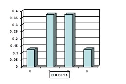
- The Number of girls in a family with three children:
|
Value x |
P(X=x) |
|
0 1 2 3 |
0.125 0.375 0.375 0.125 |
m = (0) (0.125) + (1) (0.375) + (2) (0.375) + (3) (0.125) = 1.5.
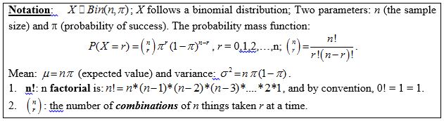
4. Bernouilli Trial & Binomial distribution
Definition: An experiment which can result in only one of two mutually exclusive outcomes (e.g., male/female, dead/alive, diseased/non-diseased,…) is called a “Bernouilli Trial”. One of the outcome is denoted “success” and the other “failure”; probability of success is known, let’s say, p (e.g., p = 0.5; 0.25); probability of failure is 1-p. This probability distribution is usually denoted by Be(p).
Consider n independent trials from an experiment with only two possible outcomes, at each trial, which are denoted as “success” and “Failure”. Furthermore, the probability of a success is the same at each trial, denoted p, and hence the probability of a failure at each trial is 1-p. Let the variable X be the number of successes in n trials. Then, the probability distribution of X is known as the Binomial distribution.
1. Example of the number of girls in a family with three children: n = 3; p = 0.5, as seen above; Mean = (3) (0.5) = 1.5; variance = (3) (0.5) (0.5) = 0.75 (= 3/4).
2. Example of white blood cells: n = 3; p = 2/3; Mean: = (3) (2/3) = 2; variance: = (3) (2/3) (1/3) = 2/3.
3. Example of recovery from delicate surgery: n = 20; p = 1/4 = 0.25; X ~ Bin(20, 0.25);
(a) P(X < 3) = P(X = 0 or X = 1 or X = 2) = P(X = 0) + P(X = 1) + P(X = 2) = 0.09126
(b) P(X > 5) = 1- P(X 5) = 1- P(X = 0 or X = 1 or X = 2 or X = 3 or X = 4 or X = 5) =
1- (P(X = 0) + P(X = 1) + P(X = 2) + P(X = 3) + P(X = 4) + P(X = 5)) = 0.38283
Note: There exists as well a freeware program, StaTable developed by Cytel Software Corporation, that computes probabilities for various probability distributions. (https://lo.unisa.edu.au/pluginfile.php/986155/mod_folder/content/0/setup.exe?forcedownload=1).
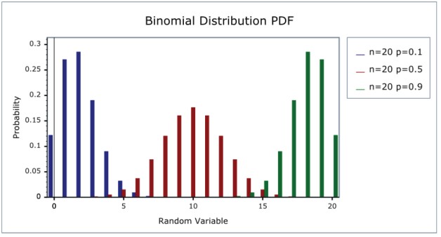
Some examples of Binomial probability distributions:
Keep the success fraction p fixed at 0.5, and vary the sample size (n)

Alternatively, we can keep the sample size fixed at n = 20 and vary the success fraction p:
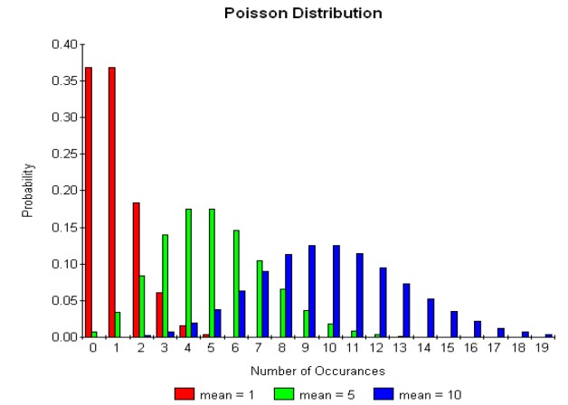
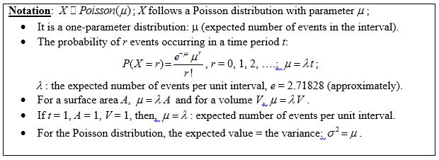
5. Poisson distribution
Examples
The Poisson distribution is applicable for discrete variables counting the number of events occurring in a certain interval of time (number of emergency calls over a day, a week, a year,…, etc.) or unit of measurement such surface area (number of bacterial colonies on agar plate, number of deaths in a given unit of intensive health care,…., etc.) or volume (number of E. coli bacterial colonies in 1 mL of water sample).
Assumptions underlying the Poisson distribution
- The probability of observing the event of interest is directly proportional to the length of that interval (interval of time, or surface area, or volume,….,etc.);
- The number of events occurring per unit of time or surface area or volume is the same throughout the entire interval;
- If an event occurs within one subinterval, it has no bearing on the probability of an event in the next subinterval and the number of events reported in any two distinct intervals are independent random variables.
Examples
(1) Consider the distribution of the number of deaths attributed to typhoid fever over a period of time, say 1 year (Infectious Disease).
(2) Consider the distribution of the number of bacterial colonies growing on an agar plate (Bacteriology).
Example 1 Infectious disease:
Suppose that the number of deaths attributable to typhoid fever over 1-year period is Poisson with parameter m = 4.6 (that is, there are, on average, 4.6 deaths per year attributable to typhoid fever). What is the probability of getting (a) no deaths, (b) at least 1 death, over a 6-month period?

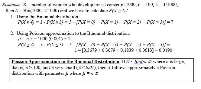
Example 2 Breast Cancer:
Suppose that we are interested in the genetics susceptibility to breast cancer. We find that 4 out of 1000 women aged 40-49 whose mothers have had breast cancer develop breast cancer over the next year of life. We would expect from large population studies that 1 in 1000 women of this age group will develop a new case of the disease over this period of time. How unusual is this event?
Visual examples of Poisson distributions