Introduction to R
| Site: | learnonline |
| Course: | Research Methodologies and Statistics |
| Book: | Introduction to R |
| Printed by: | Guest user |
| Date: | Sunday, 31 May 2026, 9:24 AM |
Description
Table of contents
- 1. What is R?
- 2. How does R work?
- 3. Getting to know the R interface - objects
- 4. Entering data
- 5. Importing data into R
- 6. Creating new variables
- 7. Accessing specific elements of a dataframe
- 8. Logical operators and functions
- 9. Subsetting dataframes
- 10. Help
- 11. Saving your work
- 12. Factors – recoding variables
- 13. Summarising data
- 14. Basic plotting
- 15. Test of Normality
- 16. Comparing means
- 17. Regression
- 18. Comparison of regression models
- 19. Correlation
- 20. Confidence Intervals
- 21. Combining dataframes
- 22. The powerful “merge” function
1. What is R?
“R” is a very powerful statistical and graphing package originally developed in 1996 as a free version of S-Plus. Since then the original team has expanded to become known now as “R core group” (https://www.r-project.org/contributors.html) the include dozens of individuals from all over the globe. R is a GNU project, which means that it is “Open Source” and is available as free software under the terms of the Free Software Foundation’s GNU General Public License – which is a key advantage over many other statistical software. In addition it is available for a variety of operating systems, including Windows, Apple MacOS as well as several flavours of Linux. R is very powerful: it easily matches or even surpasses SAS or Stata, with over 5000 specialized modules (called “packages”) available. Researchers around the world write their own procedures in R, and there are many sites on the internet with tutorials or discussion boards where you can seek help. To get R, visit the R Project homepage (http://www.r-project.org) and follow the links.
2. How does R work?
One of the disadvantages of R is that it is essentially a computer language, and does not use a “graphical user interface” (ie. menus and buttons) like other software do. Instead, the user types commands directly into a window (the “console”) in the R software. This is often a reason for people to think that R isn’t for them! However, with a little bit of time and effort, many people find this an advantage, because once you know the commands, it is much easier and faster to work with than the menu. In addition, a series of commands can also be pre-written all together in a plain text file called a “script” which you save on your computer just like any other document. The script is then ran within R and performs the desired analysis. These scripts can be easily used again and again, or more importantly, very quickly copied and modified to analyze different data or to include different/new analyses. Using a menu-driven system requires the user to click buttons and make selections – often this is not documented anywhere other than the user’s memory. In contrast, the script serves as a permanent record of what was performed – this is a key element of “Reproducible Research” (https://en.wikipedia.org/wiki/Reproducibility) which is becoming increasingly important these days, especially in data analysis (https://www.coursera.org/learn/reproducible-research http://www.ncbi.nlm.nih.gov/pubmed/26711717). R is not alone in the use of scripts rather than menus and buttons – other software also use scripts, recognizing the advantages they afford.
There is a “sort of” graphical user interface called R Studio (https://www.rstudio.com/) which has a free version, but it isn’t anything like you’d find in Stata for example, and we won’t be using it in this course.
3. Getting to know the R interface - objects
In this course, we will be using R commands and/or scripts. It’s possible to use the built-in text editor with Windows (NotePad) or MAcOS (TextEdit) to record/store your commands as a script, although I prefer a dedicated text editor, which has additional functionality eg. very powerful find and replace features, and automatic highlighting of R commands in colours, and includes line numbers – it’s useful to easily find bits of the script later on by line number. I recommend “NotePad++”, but that's just what I prefer (it’s free!). Don't use a word processor – these often include “hidden” symbols which can interfere with R.
Other things worth noting is that R ignores extra spaces in commands, and is very much case sensitive. The variable “Age” is different to the variable “age”. R also ignores anything on a line that follows a # symbol. This is very handy, as it is possible (and highly recommended from a reproducible research perspective!) to add comments to your scripts using the # symbol. In complex scripts it's a great idea to make many comments explaining what you are doing. Then you don't have to try to remember weeks (or years!) later, and it’s much easier for others to understand what you did! It’s also important to note that R ignores spaces, so its okay to use lots of spaces to make your scripts look nice. Don't use tabs though: it’s considered poor form in writing code, and tabs can often be recorded as special characters in some text editors.
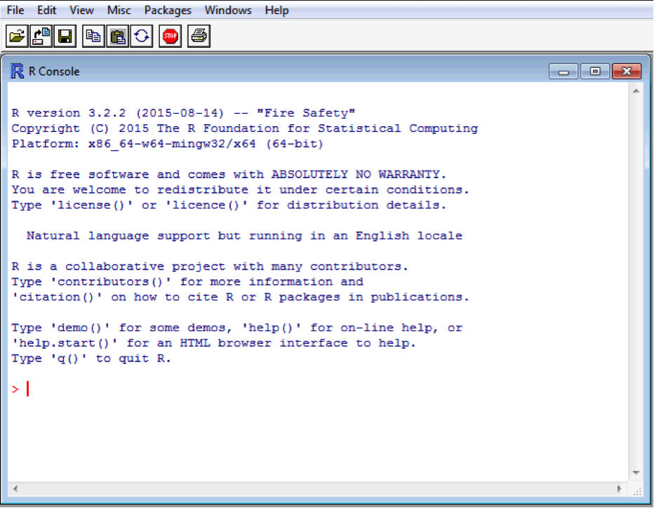
When you open R the main window will be the “console”, and it will have a “>” symbol where you start typing. To make R perform the command you gave it, you simply press the “Enter” key (often called the “Return” key) on your keyboard, at times I’ll show this with <Enter>, which means press the Enter button. For example: Open R
The prompt “>” indicate that R is ready to receive a command. Type 2 + 2 into the console, and press enter to submit the command and receive the result.
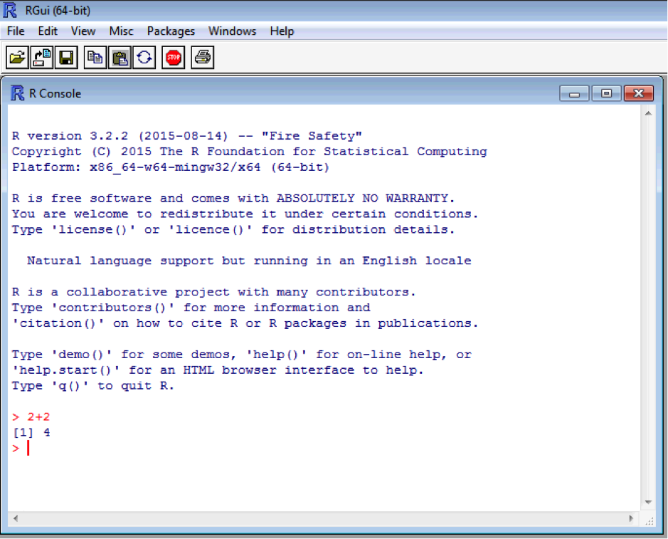
[1] indicates the first entry in the first line of the output line. This is handy for multiple line answer – but more on that later. Typing “<-” (a back arrow and a hyphen with no spaces) tells R to assign something or perform a command on an object. Assignment works from right to left. Enter these two commands:
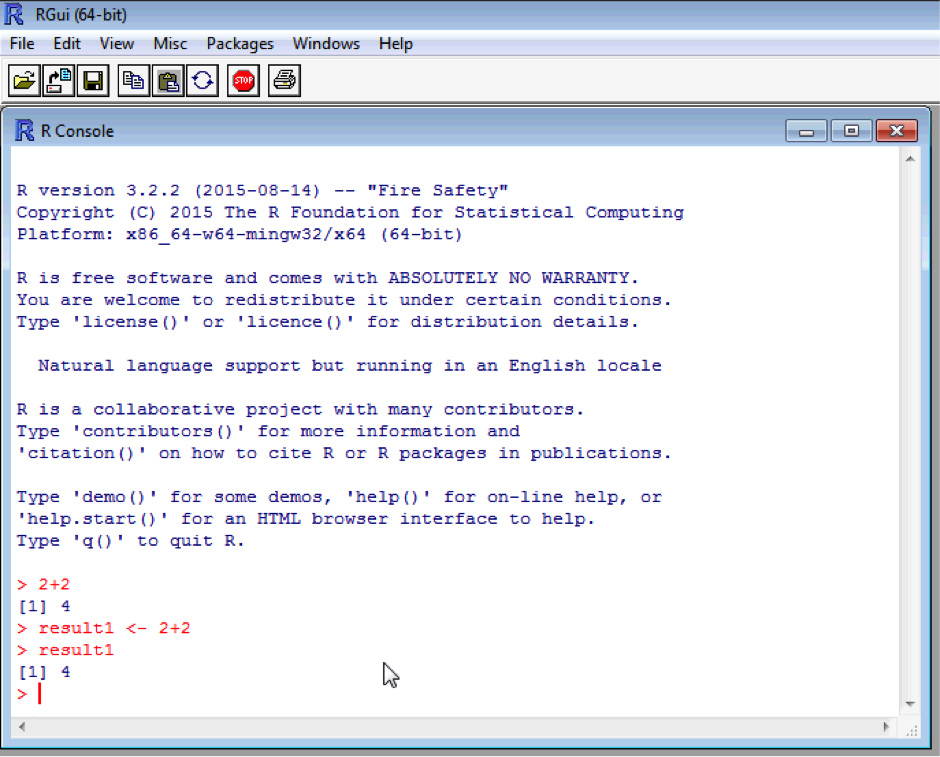
The sum of 2 and 2 has now been assigned to an object called “result1”. Typing result1 will show the contents of the object. Naturally this is a single number, 4. Again, note that R is case sensitive and so result1, Result1 and RESULT1 will all be different objects. Try typing in “Result1” and see what happens!
Ultimately you will end up with many objects in your “workspace” (ie. R’s memory). Create a second object called result2 and make it equal 4 + 4. You can list the objects in your workspace using the in built “ls()” function.
Functions are called by name followed by brackets which contain the arguments (modifiers) to the function. “ls” is called without arguments because we simply want a list of all objects in the workspace , so the brackets are empty.
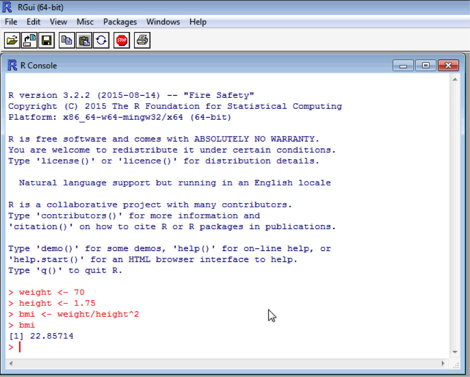
Objects can be overwritten! This is important because it allows you to update or modify an object. However, it can lead to problems if done by accident, so be careful naming objects! Say we want to add 10 to result1:
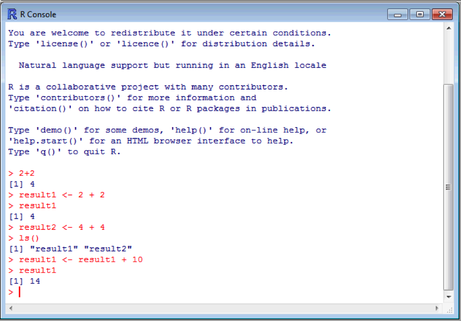
Now result1 is equal to the value 14! Quite often it’s safer to create a new object calculated form existing objects which we want to keep. For example, say we want to calculate a body mass index. We need a weight and a height, and BMI is calculated as weight/height2. Create two new objects called weight (70) and height (1.75), and one called bmi which is calculated as above (we will assume the weight is in kg and height is in metres). You’ve probably by now noticed that R will pop up suggestions for things as you type – quite handy if you forget the exact name or spelling. Don't forget to type bmi into the console to get the value of bmi!
weight <- 70
height <- 1.75
bmi <- weight/height^2
bmi
4. Entering data
So far we have entered data directly by typing. Clearly this is very time consuming, and you probably already have your data in some form of electronic format. You can import data directly into R from a variety of formats, including Excel. Things get a bit tricky when you have multiple worksheets and formulas in a Excel. However, once you start using R you will never bother to use Excel for anything more than storing raw data in a single worksheet anyway. The easiest way to enter data is to import it from a comma-delimited file. A comma-delimited (.csv) file is easily produced from an Excel spreadsheet. Just open your Excel spreadsheet in Excel to the worksheet you want to import into R, and Choose Save as -> Comma Separated Values. There is also a fantastic R package called “foreign”, which can read in to R different files from many types of statistical packages including SAS-transport files.
Example Dataset
Download the Recruits.csv file, and save it to your c:\data directory. If you double click on it, it will open in Excel. It contains data from a study of 205 military recruits. Here is what it looks like:
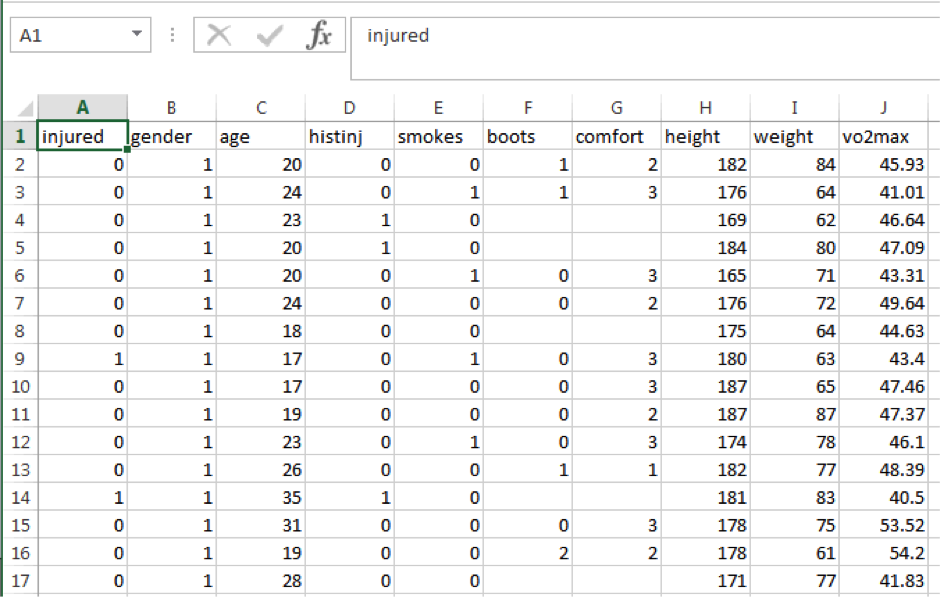
Box 1 below describes the variables:
|
Variable |
Description |
Coding |
|
injured |
Injured during training |
0=No, 1=Yes |
|
gender |
Gender |
1=Male, 2=Female |
|
age |
Age |
|
|
histinj |
Any previous lower limb injury? |
0=No, 1=Yes |
|
smokes |
Smokes cigarettes |
0=No, 1=Yes |
|
boots |
Type of boots |
0=General Purpose, 1=Taipan, 2=Other |
|
comfort |
Boot comfort score |
1=Extremely comfortable, 2=Comfortable, 3=OK, 4=Uncomfortable, 5=Extremely uncomfortable |
|
height |
Height (cm) |
|
|
weight |
Weight (kg) |
|
|
vo2max |
Aerobic fitness from initial run |
|
Being a comma-delimited (.csv) file, this file is simple plain text with the rows represented on new lines, and the columns separated by commas within each line. Try opening the Recruits.csv file in NotePad (right click > open with > NotePad).
Download the Recruits.csv file, and save it to your c:\data directory. If you double click on it, it will open in Excel. It contains data from a study of 205 military recruits. Here is what it looks like:
5. Importing data into R
A data-frame is essentially the equivalent of a spreadsheet, but it is much more powerful. A dataframe is defined by columns and rows, and each column can contain different types of data much like a spreadsheet. However, a while column can contain only one type of data, there are many different formats that can be used - including lists or even a whole new dataframe! We will keep it simple for this course and just focus on numbers or letters for now.
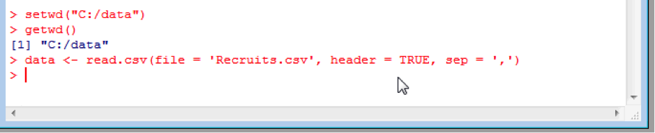
To import our data set into R, we first need to tell R where the “working directory” is. The working directory is where R will look for data and save data by default. This is done with the setwd(“<directory path>”) command. You can also check what the working directory is with the getwd() command. Please note, that file paths use forward slashes, not back slashes:
setwd(“C:/data”)
getwd()

This process also reinforces how to use functions with R, which we touched upon earlier in the list ls() function. Functions are called by name (here setwd) followed by brackets with the arguments (modifiers) to the function (here the directory path “C:/data”). Getwd is called without arguments because we just want to know what the working directory is, so the brackets are empty.
Now we tell R to import the data by creating dataframe, called eg. “data”, containing the contents of the Recruits.csv file:
data <- read.csv(file = 'Recruits.csv', header = TRUE, sep = ',', na.strings=c("",".","NA"))
The function is read.csv. The first part of the arguments (file = “ ”) says which file we wish to import. The second argument (header= TRUE) indicates whether or not the first row of the file is a set of labels (ie. column headings). The third argument (sep = ‘ ’) indicates the delimiter (in this case it's a comma as it is a .csv file). The latter two arguments are actually the default values that R would assume, and so these arguments could be left out of your command if you wish (ie. you could have just typed data <- read.csv(file = 'Recruits.csv'). However, let’s say you has a text file where the delimiter was a semi colon “;”. Then you would replace the colon with a semi colon:
data <- read.csv(file = 'Recruits.csv', header = TRUE, sep = ';')
Or perhaps there was no header line containing the column labels:
data <- read.csv(file = 'Recruits.csv', header = FALSE, sep = ',')
another useful argument is na.strings, which allows you so specify what defines a missing value. The default is no entry at all in the data (hence this argument wasn’t used above). However, people often choose to use all sorts of symbols, for example NA or a period – or worse yet, several different symbols! You can specify these yourself, for example:
data <- read.csv(file = 'Recruits.csv', header = TRUE, sep = ',', na.strings=c("",".","NA"))
If we wish to view the contents of the dataframe, we can simply type in its name as before. However, with a large dataframe this will be very long listing, and we would have to scroll a long way back to the top to see the headings. To have a quick look at the data we can use the head and tail commands to view the beginning and end of the dataframe, respectively.

Now you can see the imported data. Note that missing values are shown as “NA”. These functions have the default arguments of 6 lines of data. To modify this include the argument specifying the number of lines you want to see. For example, to see 10 lines of data, type:
head(data, 10)
If you wanted to find out more about the dataframe, for example to check how many entries there are, you can do this using the dim or str functions:

As we can see, there are 205 entries (rows) and 10 variables (columns), just like we expected when we looked at the raw data in Excel. The str function also lists the variable names, denoted with a $ sign, and gives the first few values in the data frame.
6. Creating new variables
Variables inside a dataframe are accessed in the format <dataframe>$<variable>. If we wished to calculate the BMI for all 205 subjects in the dataframe, we can follow the same procedure as above, but by creating a new column in the data frame, rather than a new object:
data$bmi <- data$weight/(data$height/100)^2 # note correct height to m from cm
head(data)
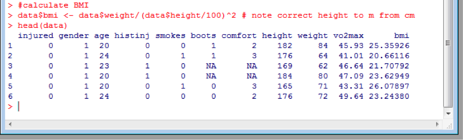
Note that here I used the # symbol to insert a comment clarifying what was done, and that importantly I did correct the height to metres from centimetres.
7. Accessing specific elements of a dataframe
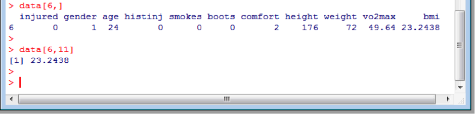
You can easily access specific rows or columns individually, or even specific elements, using the columns and row indices. For example, to access the sixth subjects data alone:
data[6,]
or the sixth’s subjects BMI (column 11) only:
data[6,11]
Note the use of square brackets.
As discussed above, accessing a column can be done by name directly by referring to the column name directly using the <dataframe>$<variable> method. For example, to access just the BMI column:
data$bmi
8. Logical operators and functions
Besides the standard format of mathematical notation common to many software (addition is +, subtraction is -, multiplication is *, division is /, and raising to a power is ^), the following list of logical operators is useful.
|
Operator |
Meaning |
|
== |
Equal to (note it is two equals signs with not space) |
|
!= |
Not equal to |
|
> |
Greater than |
|
< |
Less than |
|
>= |
Greater than or equal to |
|
<= |
Less than or equal to |
|
& |
Boolean “and” |
|
Vertical line “|” |
Boolean “or” |
Some other useful mathematical functions are:
|
Function |
Meaning |
|
max(x) |
Minimum value |
|
min(x) |
Not equal to |
|
sqrt(x) |
Square root |
|
ln(x) |
Natural logarithm |
|
exp(x) |
e raised to the power of x |
|
log(x) |
Natural logarithm |
|
log10(x) |
Logarithm base 10 |
|
abs(x) |
Absolute value |
|
round(x) |
Round to the nearest whole number |
|
sum(x,y,z) |
Sum of x, y and z |
Note that “x” (or y or z) in the above table could be a number or a variable in the dataframe, for example try max(data$age) to find the maximum age in the dataset. They can also be combined. For example, finding the square root of the sum of the ages would be:
sqrt(sum(data$age))
and should return a result of 37.16181
9. Subsetting dataframes
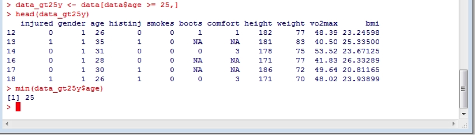
To subset a dataframe, one can use a variety of the logical operators described above. For example, we might want to subset the data for to contain only data from subjects over 25 years of age. We might also want to make this a separate dataframe so as to not overwrite our original data, and then check this to make sure that the command was carried out successfully by using the minimum age using the min function on this new data frame:
data_gt25y <- data[data$age >= 25,]
head(data_gt25y)
min(data_gt25y$age)
The above method subsets the entire data frame. If we wanted to just subset the variable “comfort” to show only data which rated their boots as uncomfortable or worse (ie. >=4):
data$comfort[data$comfort >= 4]
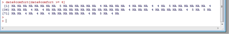
Which shows that very few subjects found their boots uncomfortable or worse, but the large number of “NA’s” also shows that there were a large number of subjects who didn’t report a value for comfort at all! These NA or missing values can cause problems. Try to calculate the median comfort rating. Then include the argument “na.rm=TRUE” (remove NA values = true):
median(data$comfort)
median(data$comfort, na.rm=T)

10. Help
Note that R has extensive help facilities. This is achieved by using the “?” command followed by the topic you help with. This will then automagically open a browser window with the help topic. For example, type
? mean
Towards the end of the help document, you will find examples, which is the first place I usually go to.
There are also a huge number of web sites with tutorials / videos / discussion boards. Google even understands what “R” means, so often I simply add “in R” to the end of the search terms that I need help with, and am usually pretty happy with the results.
In no particular order, the following are a few web sites that you might like to visit:
http://www.gardenersown.co.uk/education/lectures/r/index.htm
http://www.r-bloggers.com/how-to-learn-r-2/
If you visit these sites, you’ll probably notice that they often demonstrate different ways of doing the same thing. Everybody has their own style, and you’ll develop yours as you go along.
11. Saving your work
You can get R to save all of your commands and output into a “workspace” file ( with an .Rdata file extension). Personally I don’t do this, as it is often a large file, and in any case, I have saved by commands as a script so that I can easily run them again and return to where I was very quickly. You can find the script that I used for this course file here (right click and save Scripts.txt or Scripts.r) which contains everything in the course. Just download it and open it in NotePad or whatever text editor you prefer. Then simply copy the commands you wish to run, and paste them into R and hit <enter> on your keyboard if needed.
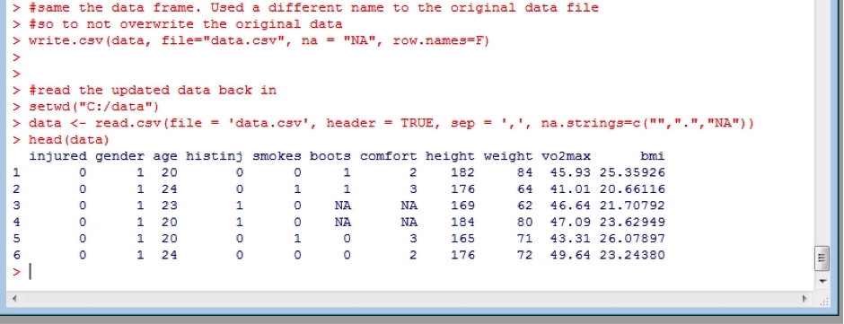
It’s also a good idea to save a dataframe once you have what you want. Then you can reload it rather than have to re-calculate things again, to save time (although R is very fast). This is done using the write.csv function:
write.csv(data, file="data.csv", na = "NA", row.names=F)
Note, I have used the argument row.names=FALSE. This is because when importing a data file, R automatically sequentially gives each row a number starting at 1. Naturally we don’t what to include those row numbers in our data file when we save it! I have also included specifying the NA values to be saved as “NA” – you could change this to whatever you wish to use. Now we can easily re-read in our saved data and start from here in the future, rather than having to start the process from the beginning (as shown earlier):
setwd("C:/data")
data <- read.csv(file = 'data.csv', header = TRUE, sep = ',', na.strings=c("",".","NA"))
head(data) #checking it loaded and looks good
Note I have also set the working directory, to make sure that its correctly set in case I decide to only run the script from this point onwards.
12. Factors – recoding variables
Factors in R represent categorical data and are important in plots, data summaries and statistics. By default R will import text data as factors. However, often the data we have uses numbers to represent different categories. For example, gender is currently coded 1 or 2 to indicate Male and Female, respectively. To check this, try the unique command for the gender variable:
unique(data$gender)
Factors have levels (names) and levels have an order. It’s easy to accidentally mix them up. The safest way I find to do this is to
(i) create a new variable to play the role of the factor (eg genderf)
(ii) very clearly declare the text descriptors
data$genderf[data$gender == "1"] <- "Male"
data$genderf[data$gender == "2"] <- "Female"
(iii) make this new variable a factor
data$genderf <- as.factor(data$genderf)
I also like to check that things are how they are supposed to be. I simply create a new object (Factor_summary) and make a table summarising the original numerical coding against the new text coding.
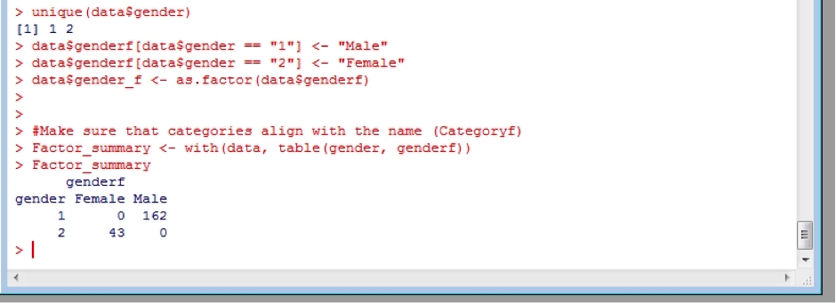
As you can see the only entries for the factors “Male” or “Female” correspond to the original 1 or 2 identifiers, respectively.
|
Exercise: Assign text-based factors to the remaining categorical variables. |
13. Summarising data
To get a quick summary of the data you can use the summary(<dataframe>) function, or for a single variable summary(<dataframe$variable>). For example, created a new object and obtain a basic summary of the overall dataset:
Summary_stats_basic <- summary(data)
Summary_stats_basic
Or just summarise the BMI data:
Summary_stats_bmi_basic <- summary(data$bmi)
Summary_stats_bmi_basic
This is limited in that it can’t easily separated (faceted) by factors. For example, separate the summary of BMI by gender. There is a very useful add-on package to R called “doBy” which, which can be easily downloaded and installed going to the Packages menu -> Install Packages and scrolling down to “doBy”, and selecting install. If R asks for a “CRAN mirror” (ie. the site you wish do download a package from) my recommendation is one from inside Australia – although hey are all approved by the R Project Group.
Once installed, you need to load the package you wish to use. This is achieved by entering the command library(<package name>); in this case:
library(doBy)
Sometimes a package will depend upon another package (R will warn you of this) and thus this requires you to install that package also. If this is the case, simply repeat the process to install all required packages. The good news is once you have installed a package you won’t need to do it again in the future.
Using doBy, you can “facet” the statistics for a specific variable by different factors (denoted by the first argument) and specify which statistics you would like in the summary (denoted by the FUN=c() argument, and also. For example, create an object “Summary_stats_boots” and then summarise the comfort by boot type and gender:
Summary_stats_boots <- summaryBy(comfortf~bootsf+genderf, FUN=c(length, median, mean, sd, min, max),data=data)
Summary_stats_boots
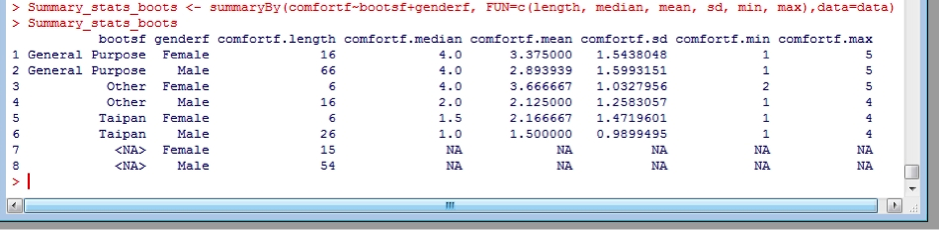
Note that I used the factors for boots (bootsf) and gender (genderf) – this way I get the understandable name, rather than the original number format. You would probably like to save this result for use later, for example in a paper you are writing. This is achieved the same way as you saved the data before, except this time the dataframe is Summary_stats_boots.
write.csv(Summary_stats_boots, file="Summary_stats_boots.csv", na = "NA", row.names=F)
You can then open the file you created and copy/paste the information you want.
|
Exercise: Summarise BMI by gender and smoking status. Save it as a csv file for later use. |
14. Basic plotting
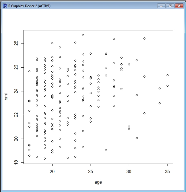
R comes with built-in plotting functionality, and interprets the data to some extent depending upon the nature of the data you are attempting to plot. For example, plotting BMI versus age generates a scatter plot as both variables are numerical.
plot(bmi~age, data=data)
Now you will notice that suddenly a new window opens up containing the plot:
You can colour the symbols as well if you wish, using the argument col=“..”
plot(bmi~age, data=data, col="blue")
To save this plot the following command is used:
dev.copy(png, ' bmi_v_age.png')
dev.off()
Where bmi_v_age.png is the name you wish to give to the picture file. This will save the plot as a “png” file, which is readable by many different software. The file will appear in your working directory.
Similarly, plotting BMI versus gender results in a (fairly meaningless) scatter plot. In contrast, a bar and whiskers plot results from plotting BMI versus genderf , as genderf is a factor this makes for a much more meaningful plot:
plot(bmi~genderf, data=data)
There are many arguments for modifying plots. Here are a few:
horiz=TRUE – rotating a plot
col="lightgreen" – changing the colour of the data
xlab="Gender" – defining the x-axis label
ylab="BMI" - defining the y-axis label
main="BMI by gender" – giving a title to the plot
There are many more option, just type ?plot for help within R. There is also a much more powerful plotting package called ggplot2, which is worth looking into.
15. Test of Normality
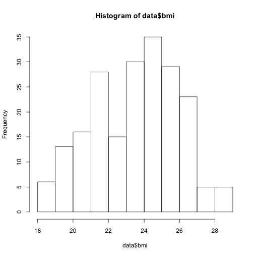
For a quick look at the shape of a distribution, try hist. For example,
hist(data$bmi)
Using arguments, you can control the number of bins and colour of the plot:
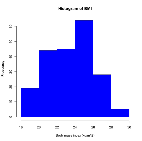
hist(data$bmi, breaks=5, col="blue")
Add a proper x-axis label (xlab = “..”) and a heading (main = “..”):
hist(data$bmi, breaks=5, col="blue", xlab="Body mass index (kg/m^2)", main="Histogram of BMI")
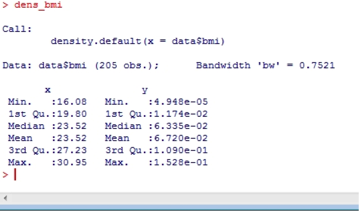
Alternatively you might like to see a density plot. First you must determine the density data, by creating an object (which I have called “dens_bmi” but you could call it what you like). Then plot the desity data.
dens_bmi <- density(data$bmi)
plot(dens_bmi)
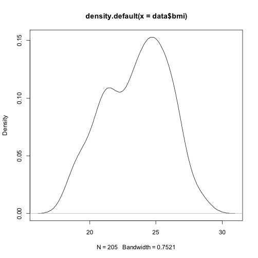
Again, you can give the plot a better heading, and colour it:
plot(dens_bmi, main="Density distribution of BMI", col="blue")
You can also ask for the density data by calling the object you just created
dens_bmi
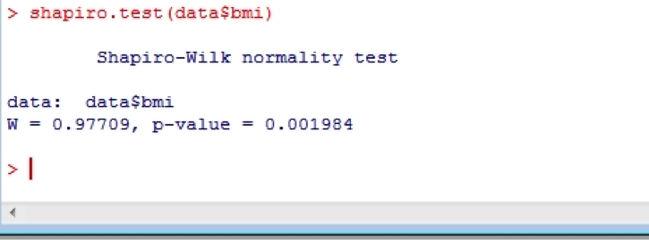
Or perhaps you’d like a more formal test? If so, you can use the Shapiro- Wilk statistic:
shapiro.test(data$bmi)
16. Comparing means
Independent samples t-tests are easy in R. Try:
t.test(bmi ~ gender, var.equal = TRUE, conf.level = 0.95, data=data)
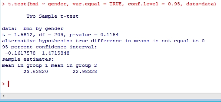
This uses the confidence level of 0.95 (conf.level = 0.95) which is the default, but you could use 0.99 if you like. Note that this test assumes equal variances (var.equal = TRUE), which is again the default, but you could change this to FALSE if need be. To test whether or not the variances are equal, use:
var.test(bmi ~ gender, data = data)
There is also the Fligner-Killeen test of homogeneity of variances, which a non-parametric test and apparently robust against departures from normality:
fligner.test(bmi ~ gender, data=data)
Oneway analysis of variance is relatively straight forwards. However, this is best done by creating an object for the results of the ANOVA, and requires that the grouping variable be a made into factor. For example for a comparison of BMI be boot comfort rating, we would use comfortf as it is a factor, and an object “anova_bmi_comf” to store the results:
anova_bmi_comf <- aov(bmi ~ comfortf, data = data)
anova_bmi_comf
summary(anova_bmi_comf)

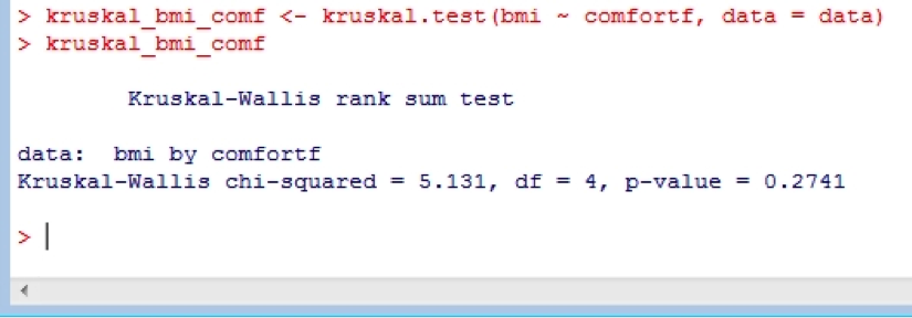
Non-parametric versions of the t-test and ANOVA are also available. For example:
kruskal_bmi_comf <- kruskal.test(bmi ~ comfortf, data = data)
kruskal_bmi_comf
17. Regression
Regression is performed in R using the linear model function lm(). This can perform single and multiple linear regression analyses. Similar to the other analyses, it’s best to create an object to store the results, and then ask for a summary. Note that we should use the factors we created earlier for boot type (bootsf) and gender (genderf). Suppose we want to know whether age, gender and type of boots can predict boot comfort score:
fit_comfort_age_boots_gender <- lm(comfort ~ age + genderf + bootsf, data = data)
summary(fit_comfort_age_boots_gender)
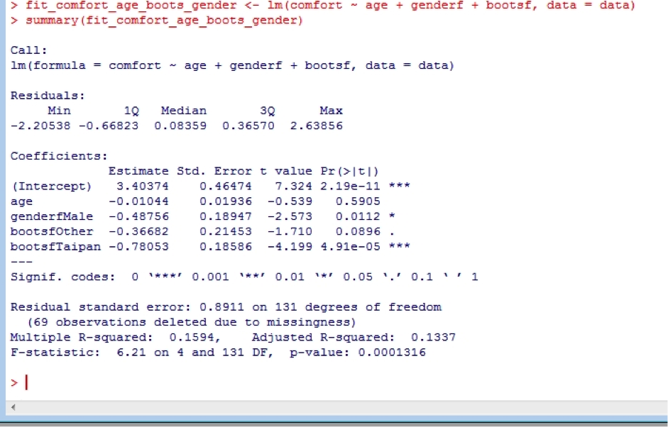
We see that overall, the type of boot worn is strongly associated with boot comfort. Interestingly, we see that female recruits give lower comfort scores than males. This is because when this study was undertaken in about 2000, female boots were actually made from male boots lasts, and so provided a sub-optimal fit. This has now been fixed, and female recruits have their own lasts.
Other useful aspects of the analysis include:
coefficients(fit_comfort_age_boots_gender) # model coefficients
confint(fit_comfort_age_boots_gender, level=0.95) # Confidence Intervals for model parameters, here set to 95%
fitted(fit_comfort_age_boots_gender) # predicted values
residuals(fit_comfort_age_boots_gender) # residuals
anova(fit_comfort_age_boots_gender) # anova table
vcov(fit_comfort_age_boots_gender) # covariance matrix for model parameters
influence(fit_comfort_age_boots_gender) # regression diagnostics
To undertake regression diagnostics, try this:
layout(matrix(c(1,2,3,4),2,2)) # optional 4 graphs/page
plot(fit_comfort_age_boots_gender)
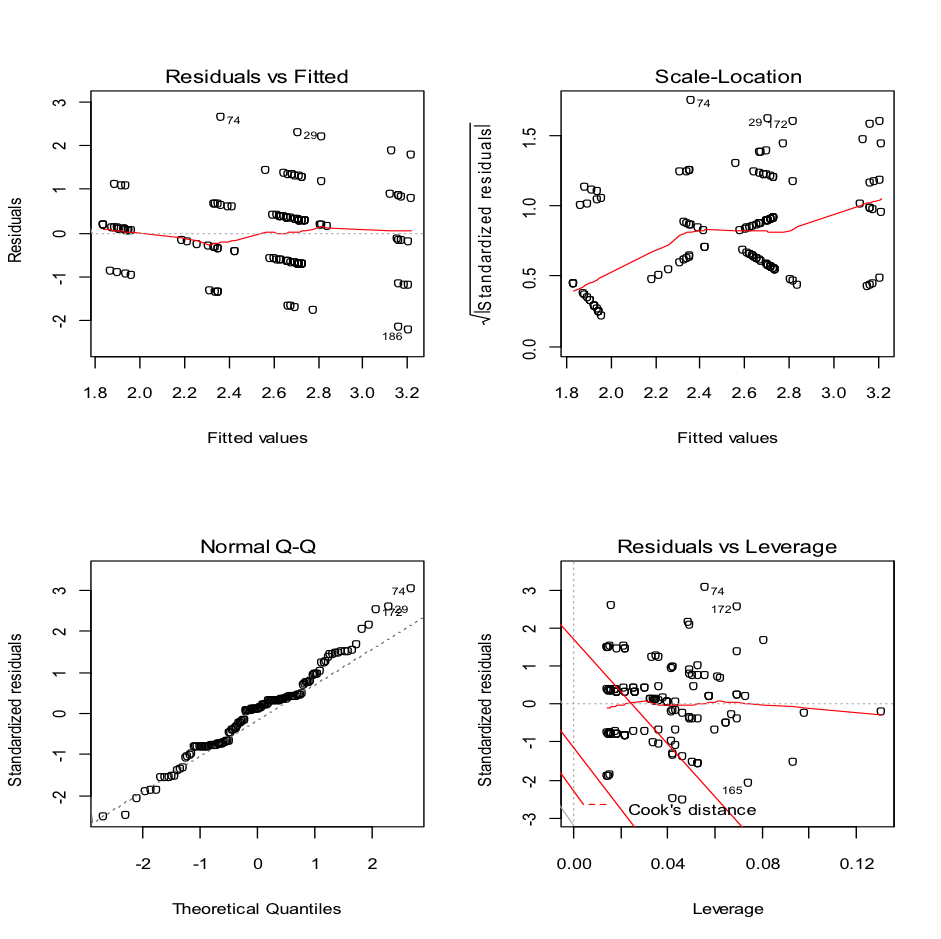
Which looks reasonable, but we can also undertake a Shapiro-Wilks test on the residuals to check if they are normally distributed. First you will need to create an object containing the residuals. This is done using the command we used above, but making it produce and store the result as an object. the residuals
fit_res <- residuals(fit_comfort_age_boots_gender)
shapiro.test(fit_res)
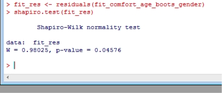
Which shows that the residuals aren’t normally distributed, but this isn’t uncommon with smaller datasets.
18. Comparison of regression models
Often we wish to compare regression models that are nested in order to see if it was worthwhile adding a new predictor variable. Comparison of nested models is performed using the anova() function. For example, we might wish to see whether age can predict vo2max in our data, and then compare that to when age and gender are used as predictors. Let’s have a go. Make sure you put the more complex model first in the anova function.
fit_vo2max_age <- lm(vo2max ~ age, data = data)
summary(fit_vo2max_age)
fit_vo2max_age_gender <- lm(vo2max ~ age + gender, data = data)
summary(fit_vo2max_age_gender)
anova(fit_vo2max_age_gender, fit_vo2max_age)
Alternatively, the Likelihood-ratio test can be used via the lrtest function. However, this requires the “lmtest” and “zoo” (which lmtest depends upon) packages, so you will need to install them as described earlier for the doBy package. Make sure you put the more complex model first in the lrtest function.
Lrtest(fit_vo2max_age_gender, fit_vo2max_age)
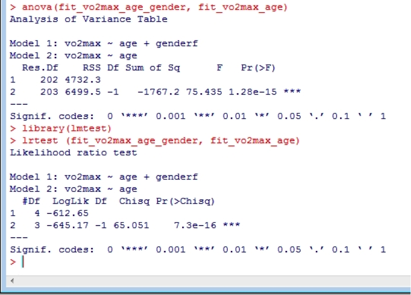
Both comparisons clearly show that it was definitely worthwhile adding gender into the model.
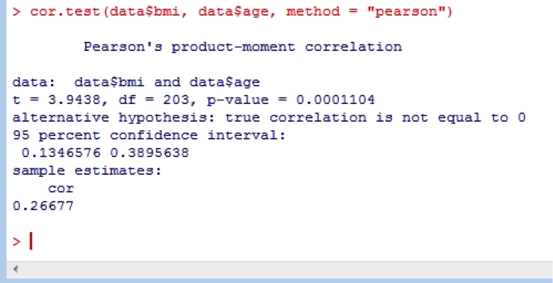
19. Correlation
Correlation is easily undertaken in R using the cor.test function. The arguments use = “..” specifies the handling of missing data with the options of all.obs (assumes no missing data - missing data will produce an error), complete.obs (listwise deletion), and pairwise.complete.obs (pairwise deletion); method = “..” specifies the type of correlation (pearson, spearman or kendall).
cor.test(data$bmi, data$age, method = "pearson")
20. Confidence Intervals
Although there are packages that can calculate confidence intervals, the standard installation of R does not. However they are easily calculated using your own code. For example:
CI <- 0.975 #95% CI
mean <- mean(data$bmi, na.rm=T)
stdev <- sd(data$bmi, na.rm=T)
n <- length(data$bmi)
error <- qt(0.975,df=n-1)*stdev/sqrt(n)
lowerCI <- mean-error
upperCI <- mean+error
mean
stdev
lowerCI
upperCI

|
Exercise: Write you own code to calculate the standard error of the mean for BMI. |
21. Combining dataframes
The ability to combine datasets from different original files is often a difficult and poorly documented process. It usually comes down to opening the files and “copying and pasting” the data from one file to another. From a reproducible research perspective this is very poor practice as there is no real documentation. In addition, it is tedious and fraught with the risk of mistakes. These issues are magnified if it is a process that is repeated often, for example merging individual files of each subject in a trial. Using R to merge or combine datasets obviates many of these problems (i) a script is the source documentation, (ii) a script cannot suffer from errors of copy/paste nature, (iii) a script can be easily ran repeatedly and/or (iv) modified to do the same or similar job for other datasets (iv) if a mistake is noted (see point (i)), or more data comes in, then the script can be fixed and re-ran with very little effort. These are especially useful properties when it comes to merging data.
Binding columns (cbind)
The simplest process is combining a new dataset which contains new variable(s) we wish to added to corresponding data original dataset. In other words joining two dataframes by column – obviously they need the same number of rows. For example, the eye colour of the subjects in the data we have been working with in this course. Download the IDdata.csv file which contains subject ID’s and eye colours. The original recruit’s data didn’t have subject ID’s in it, so we assume they are match correctly. Import it into R and then have a look at it:
head(IDdata)
str(IDdata)
unique(IDdata$eye)
plot(ID ~ eye, data=IDdata)
These functions and simple plot show that there are 205 entries and there are 3 values for eye. These are 1=Blue, 2=Brown, 3=Other. If you haven’t done so re-read in your latest saved version of the recuirts dataframe (saved as data.csv). Now we can bind the two dataframes using the cbind(<dataframe1, dataframe2, dataframe3, etc…) function:
data <- cbind(IDdata, data)
head(data)
Now assign some factors to give eye colour some meaning:
unique(data$eye) # checking that there are still only 3 values. Yes I am paranoid
data$eyef[data$eye == "1"] <- "Blue"
data$eyef[data$eye == "2"] <- "Brown"
data$eyef[data$eye == "3"] <- "Other"
data$eyef <- as.factor(data$eyef)
Factor_summary <- with(data, table(eye, eyef))
Factor_summary
head(data)
plot(ID ~ eyef, data=IDdata)
Now save the new data, lets give it a new name when we save it (just to make sure you can!):
write.csv(data, file="data_eye_ID.csv", na = "NA", row.names=F) # saving the new updated data
Binding rows (rbind)
The next case is simply joining sets of data which are identical in the variables they contain. For example, sets of data from several subjects. In this example we will pretend that we obtained the original Recruits.csv data in two halves – say from two trial sites. Download the Recruits1_100.csv and Recruits101_205.csv files, then read them in and check them out a little bit.
data1_100 <- read.csv(file = 'Recruits1_100.csv', header = TRUE, sep = ',', na.strings=c("",".","NA"))
data101_205 <- read.csv(file = 'Recruits101_205.csv', header = TRUE, sep = ',', na.strings=c("",".","NA"))
head(data1_100)
head(data101_205) #make sure the headings match
now bind them together using the rbind(<dataframe1, dataframe2, dataframe3, etc…) function and do a little bit of data integrity checking:
data1_205 <- rbind(data1_100, data101_205)
dim(data1_100)
dim(data101_205)
dim(data1_205)
dim(data) # check lengths match /add up as expected to the 205 of the original data
You might notice that the combined dataframe (data1_205) has more columns than the original data (data) – this is because earlier we created several factors. If you compare the dataframes using the head() commands, you’ll see the extra factor columns.
22. The powerful “merge” function
Merging dataframes is even more powerful. This process involves combining (merging) dataframes that share both common and different variables (columns) as well as some matching rows. For example, a trial may have measured blood concentrations of a drug as well as the effect of the drug eg. heart rate. These data may have been collected at different times after the dose and the information was stored in separate files. For example, one dataset pertains to the concentrations another to the effect on exercise-induced heart rate. Not all of the collections were the same time in each subject or measurement (concentration or effect). Naturally it’s best to have these key data in a single dataframe, and probably ordered by subject ID and sequentially in time. Doing so in Excel, for example, would involve a lot of copying and pasting, re-ordering, sorting, with each step prone to errors and very time consuming. The merge(dataframe1, dataframe2, dataframe3, etc) makes this very simple.
In this case we will merge some drug concentration-time data and some effect-time data. The effect is heart rate (hr). Import the concentration_data.csv and effect_data.csv (link this please) files into R:
conc_data <- read.csv(file = 'concentration_data.csv', header = TRUE, sep = ',', na.strings=c("",".","NA"))
head(conc_data)
hr_data <- read.csv(file = 'effect_data.csv', header = TRUE, sep = ',', na.strings=c("",".","NA"))
head(hr_data)
all_data <- merge(conc_data, hr_data, all = TRUE)
head(all_data)
Notice that the data from both subjects now includes both the variable conc (concentration) and hr (heart rate), and that they are ordered sequentially by time.
|
Exercise: Create plots of concentration versus time and heart-rate versus time, colour the symbols by subject ID, and save the plots. Do this for both the original data and the merged data. Satisfy yourself that they are identical. |