Introduction to SPSS
| Site: | learnonline |
| Course: | Research Methodologies and Statistics |
| Book: | Introduction to SPSS |
| Printed by: | Guest user |
| Date: | Thursday, 21 May 2026, 11:05 AM |
1. Introduction
Welcome to the Introduction to SPSS module!![]()
The aim of this module is to introduce you to the SPSS software, including navigating the program interface and using syntax to manage and analyse data. The module will also cover how to access and undertake commonly used descriptive data analysis procedures in SPSS.
I would recommend splitting your screen with this module on one side, and the SPSS program on the other side of your screen. Even better if you have dual screens! It will be much easier to work through the module if you have visual access to both this module and SPSS (otherwise you'll constantly be flicking back and forth from one to the other).
2. Datasets and files to download
To undertake this module, you will need access to a couple of datasets and related files.
Please download and save the following files to a sensible location, where you can easily access them for the duration of this module:
1. 2016 Health and Society student health survey data (SPSS format, 36 KB): HLTH1025_2016.sav
2. 2016 Health and Society student health survey data (Excel format, 93 KB): HLTH1025_2016.xlsx
3. SPSS Health and Society student health survey data_Year (SPSS format, 4 KB): HLTH1025_2016_yr.sav
![]()
3. Part I: Introduction to the SPSS software
In this section, we will cover:
- What the SPSS software is and what it is best used for;
- How to open data (multiple ways);
- The SPSS interface; and
- Getting your SPSS files organised.
![]()
3.1. What is SPSS?
![]() SPSS (Statistical Package for the Social Sciences) is a versatile and responsive program designed to undertake a range of statistical procedures. SPSS software is widely used in a range of disciplines and is available from all computer pools within the University of South Australia.
SPSS (Statistical Package for the Social Sciences) is a versatile and responsive program designed to undertake a range of statistical procedures. SPSS software is widely used in a range of disciplines and is available from all computer pools within the University of South Australia.
It’s important to note that SPSS is not the only statistical software – there are many others that you may come across if you pursue a career that requires you to work with data. Some of the other more common statistical packages include Stata and SAS (and there are many others). The focus for this session, however, is on SPSS.
 Task: Open SPSS
Click on the Start menu (![]() ) > All Programs > IBM SPSS Statistics > IBM SPSS Statistics 21 (or whatever is the latest version number) to open the SPSS program.
) > All Programs > IBM SPSS Statistics > IBM SPSS Statistics 21 (or whatever is the latest version number) to open the SPSS program.
When you first open SPSS on your computer, you should see something that looks similar to to following screenshot:
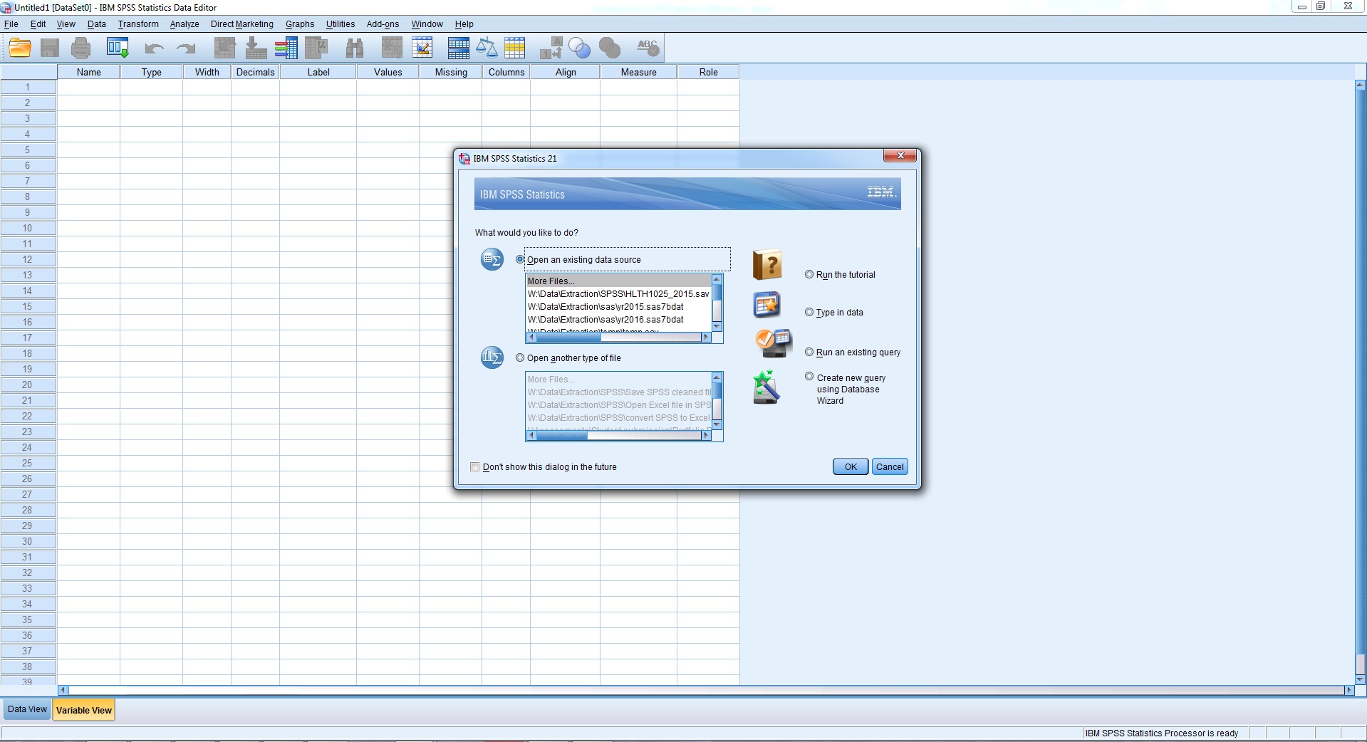
SPSS automatically assumes that you want to open an existing file, and immediately opens a dialogue box to ask which file you’d like to open. It’ll make it easier to navigate the interface and windows in SPSS if we open a file.
We’re going to open and use from data collected as part of a first-year course at UniSA, called Health and Society (H&S). The data we are going to use were collected at the beginning of 2016. So let’s first open our demonstration data set – the 2016 H&S student health survey data.
3.2. Opening data - Part 1
![]() In the active dialogue box that asks very nicely, "What would you like to do?", we are going to "Open an existing data source", by clicking the "More files ..." option and finding our way to where we earlier saved our H&S dataset.
In the active dialogue box that asks very nicely, "What would you like to do?", we are going to "Open an existing data source", by clicking the "More files ..." option and finding our way to where we earlier saved our H&S dataset.
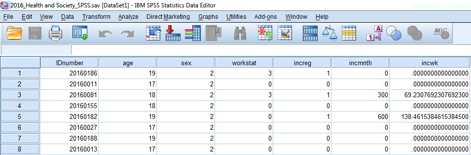
Once you have found the file you want to open, click Open and you’ll (hopefully!) see a data file in front of you that looks something like this:
The other bit you may have noticed pop up was another window, mostly blank, but with a bit of funny looking writing in it, like this:
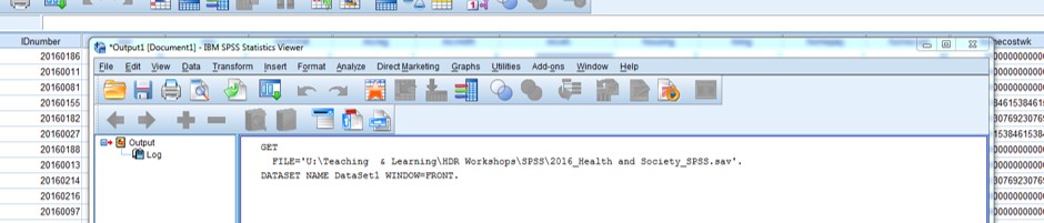
Now that we have opened a data file, SPSS automatically opens what is called an “Output Viewer” window. We’re going to talk about the SPSS interface, including this window, shortly. Next, we have an example of how to open a data file using the SPSS drop down menus.
3.3. Opening data - Part 2
![]() It can be handy to know how to open a dataset once you’re already in SPSS, using the drop down menus.
It can be handy to know how to open a dataset once you’re already in SPSS, using the drop down menus.
So far we've learned how to open an SPSS file when we first open SPSS. But sometimes you might already have SPSS open and wish to open a(nother) data file. Later on we will talk about how to use syntax files to work in SPSS, starting with opening data, but for now, here's how to open a file using the menus:
Click on the File menu at the top left of your Data Editor window, then Open > Data … :
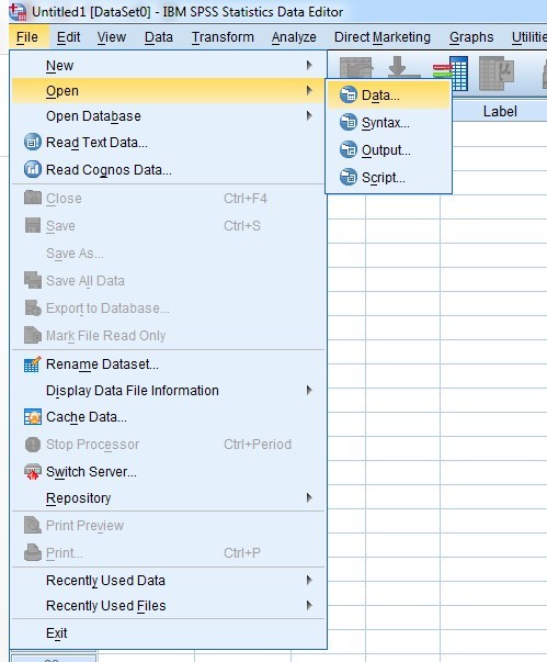
Here you can navigate to your working folder and open your data file.
3.4. Navigating the SPSS interface
Data editor window![]()
This is the window where you can see your data, and information about the variables in your dataset. It is also possible to change your data in this window, but I would strongly recommend against ever changing your data that way because things can go terribly wrong and you have no record of what you changed and how you changed it!
There are two ‘views’ for the Data Editor window:
1) Data view – you can see the actual data in your dataset for each record and each variable; and
2) Variable view – this gives a summary of each variable in your dataset, including the variable name, type, various properties of the way in which the data are stored, any label(s) for the variable itself and variable values (such as value labels for categories of sex, which in the dataset may be represented as 1 and 2, relating to male and female).
Syntax editor window
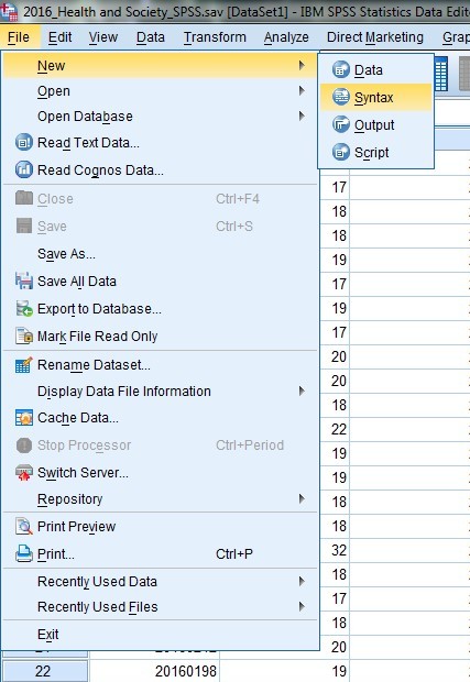
A second window in the SPSS interface is the Syntax Editor window. SPSS doesn’t automatically open a syntax file for us, so let’s open one now. Click on the File menu in the top left corner of your screen, and select New > Syntax:
The syntax window is where we can run commands (tell SPSS what we want it to do), such as opening files, editing and managing data, undertaking statistical procedures and tests, and saving files. The Syntax Editor window is essentially a file that we can use to record and save everything that we do for a particular piece of analysis, or when managing/editing a dataset.
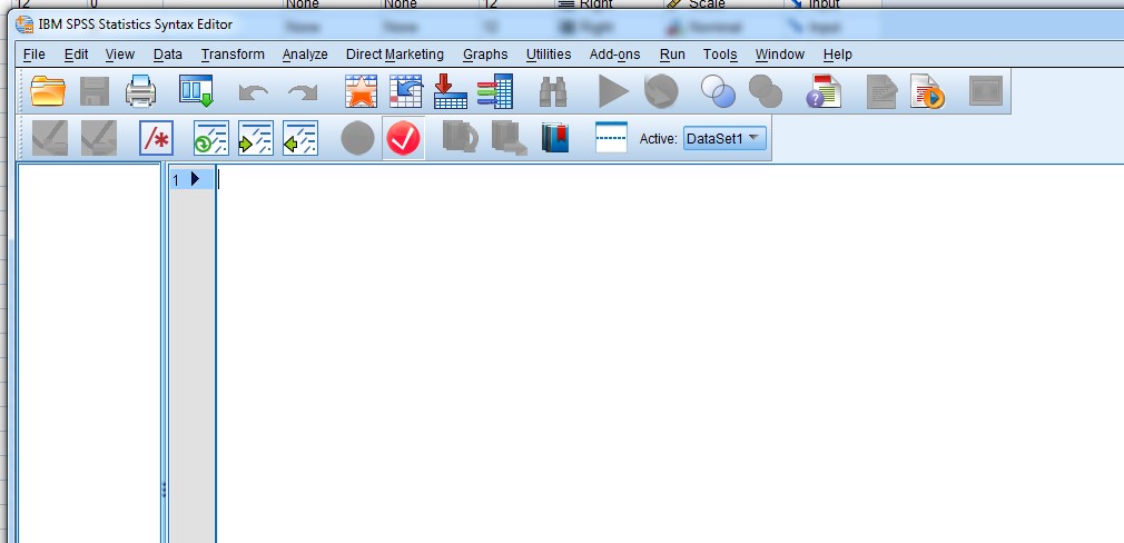
When you first open a syntax file, it looks similar to a blank Word document:
While many people feel extremely uncomfortable using syntax, and would much rather use the built-in menus (sound like you?!), in SPSS you can actually do both (use the menus and the syntax file) for many procedures. We will start off by doing this, to ease you into using SPSS syntax.
Regardless of whether you write the syntax yourself, or paste it into a syntax file from the menus, it really is best practice to use a syntax file to keep a record of all your data management and analysis procedures.
van den Berg (2013) lists six reasons you should use SPSS syntax:
- Syntax is ideal project documentation;
- Syntax can be corrected;
- Syntax can be recycled;
- Syntax gets things done fast;
- Typing syntax saves time; and
- Syntax has more options.
A little later we will cover the basics of SPSS syntax, including a bit more information on these six reasons for using it. By the end of this session, you should be well on your way to using SPSS syntax competently and confidently!
Output viewer window
Any time you do anything in SPSS – even just opening a file – SPSS will document it in the Output Viewer window. If you don’t already have an output window open, SPSS will open a new one for you, as it did when we first opened a dataset.
The output viewer window will keep a record of any and all commands you give SPSS (e.g., open a file, save a file, etc.), and is also the window in which you can view the results of any data/statistical procedures undertaken.
You can see in the screenshot below, that SPSS has made a record in the Output file that you opened a particular SPSS file:
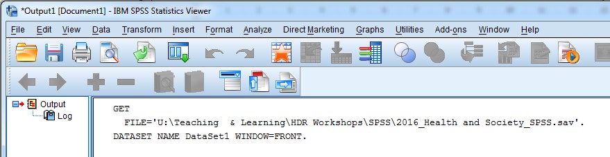
It shows us the syntax command that SPSS recognises to open a file (GET FILE), and it also shows us the structure of the syntax:
GET FILE=‘[file path\file name.sav]’.
GET FILE is the command, then there is an equals sign (=), followed by the file path and file name.sav in single quotation marks, and a full stop (.) at the end of the command. SPSS syntax always starts with the command name and always ends with a full stop (.).
The second line starting with the command DATASET NAME is a very useful piece of syntax – we’ll get to that shortly!
Similar to the Syntax Editor window, the Output Viewer window is simply a file that you can save and edit if you wish. You can also copy tables and graphs (or anything else) presented in the output file into Microsoft Word, Excel or other similar programs.
3.5. Getting organised
![]() When you’re working with data in SPSS (or any software for that matter), ideally you should keep your work organised. How you organise your work is up to you, but here are some general tips that may help make your life easier:
When you’re working with data in SPSS (or any software for that matter), ideally you should keep your work organised. How you organise your work is up to you, but here are some general tips that may help make your life easier:
- Keep all the files relating to a single ‘project’ in the one place. A ‘project could be an analysis for a chapter of your thesis or for a publication, primary data collection, data management processes, etc.
- Make sure you work is backed up. Either save it somewhere that is automatically backed up, or back it up yourself, regularly.
- Never edit your original data file. You should always keep a copy of your original data, and keep it somewhere that you won’t accidentally edit or overwrite it. You may want to keep it in a sub-folder, for instance. Sometimes we make mistakes in managing and using data, and need to go back to the original file. Storing your original data can also be an important ethical consideration.
- Label your files well, with descriptive file names.
- You may like to number them in the order that they occur in the project by placing a number at the front of the filename (a good way to do this is to number using tenfolds (10, 20, 30 …) so that you can insert files later if needed. For example, you could prefix a file with 15 if you wanted it to be run between file 10 and 20.
- Use descriptive file names so that you have a good idea what’s in there when you want to find something a year or two (or five) down the track.
Task: Organise your SPSS files
If you have never been so organised with your data sets, now is an excellent time to start! There’s really not a whole lot worse than doing a bunch of analyses using multiple datasets and having the files all jumbled in with other documents … or worse, spread all over the place in separate folders!
- Select a location on your computer, removable disk drive, or a cloud location to organise your files for this workshop.
- Use some of the tips above to label your files well, and save original data in a sub-folder (you can take copies of the original data files and save them in the main folder location).
Your folder might now look something like this:
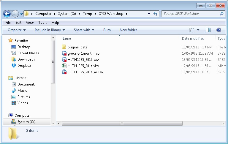
Note: the “original data” folder has a copy of all datasets (in SPSS and Excel) shown in this main folder directory.
4. Part II: Using Syntax
![]() Here is your opportunity to get familiar with using syntax (code) in a statistical software package. You may have used other statistical packages, but each one has a unique syntax. Although once you become comfortable with the idea of using syntax, it’s not so difficult to move from one program to the next and learn the unique commands and syntax structure for each.
Here is your opportunity to get familiar with using syntax (code) in a statistical software package. You may have used other statistical packages, but each one has a unique syntax. Although once you become comfortable with the idea of using syntax, it’s not so difficult to move from one program to the next and learn the unique commands and syntax structure for each.
One benefit of SPSS, is that most of the procedures accessed in the interface menus actually allow you to paste the code for those procedures into a syntax file. This can be a great way to get comfortable with using syntax. Let’s have a go at doing this now!
4.1. Using syntax to ... open and name a dataset
![]()
 Task: Paste syntax from SPSS menus to a syntax file
- Click File > Open > Data …
- Navigate to and select the file “HLTH1025_2016.sav”
- Click the Paste button (just under the Open button) to the right hand side of the dialogue box.
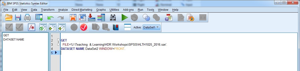
This should have done two things: 1) open a new syntax file; and 2) paste the syntax command to open the file you selected into the new syntax file. Amazing, isn’t it?! You should now have a syntax file that looks like this:
What we want to do, though, is to make sure we properly document what we have done, and save the file. This means that we can come back to it at any time in the future and know exactly what the syntax is doing, what it’s for, who wrote it, and when it was written. These are really useful bits of information to keep track of, especially if you or someone else goes back in and makes changes to the file. You can then record who has done what, and when it was done (and why!).
An important thing to know about SPSS syntax before we go any further:
- If you want to write a comment, or any sort of text that is NOT an SPSS command (telling SPSS to do something), then you need to preface your text with an asterisk (*). You also need to end your text with a full stop (.). When reading your syntax, SPSS will ignore any text within an asterisk and a full stop.
So let’s have a go at ‘commenting’ our new syntax file.
Task: Documenting using SPSS syntax files
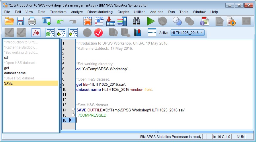
- Save your syntax file in the same place you saved your datasets (the organised version!), with a descriptive name (I’ve called my syntax file “10 Introduction to SPSS workshop_data management”).
- Have a go at documenting what the file is for, who wrote it (that’s you), and today’s date. You can see how I’ve commented my file below:
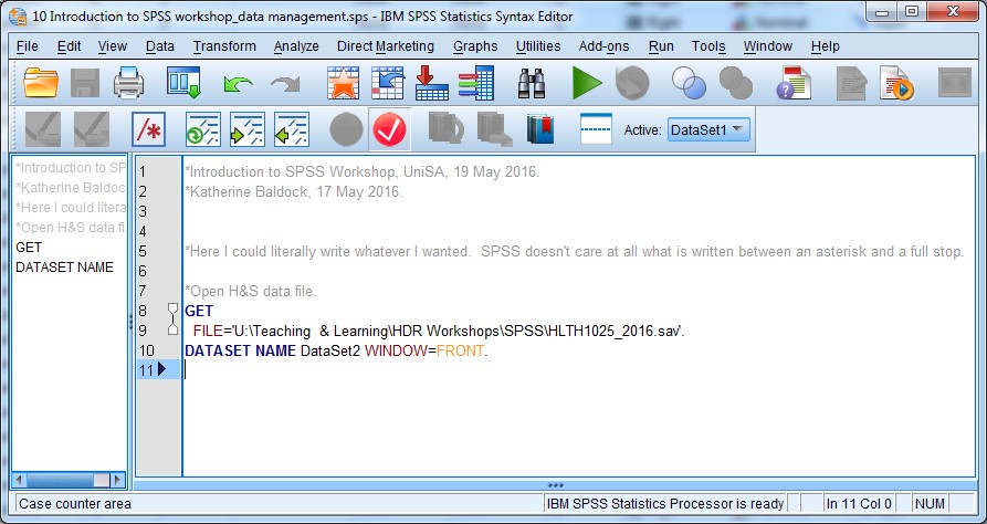
You may have noticed from the image above that SPSS colour codes its syntax – rather a neat feature I think. Commands (words that tell SPSS to do something) are in blue. Just for the record, it doesn’t matter if they’re written in all caps or not. Objects are in red, and criteria are in yellow. Text (like my comments) are in grey. We may come across some other colours as we go.
Another useful thing to do (particularly if you have multiple datasets open at once) is to label your dataset. See in the syntax above for the GET FILE procedure, there is a second line with another command DATASET NAME? This command allows us to label our dataset so we don’t mix it up with another one if we have lots open at once.
Let’s modify the dataset name so that instead of being called “DataSet 2” it’s called “HLTH2015_2016”, using the syntax as follows:
dataset name HLTH1025_2016.
Here’s what your syntax file might look like now:
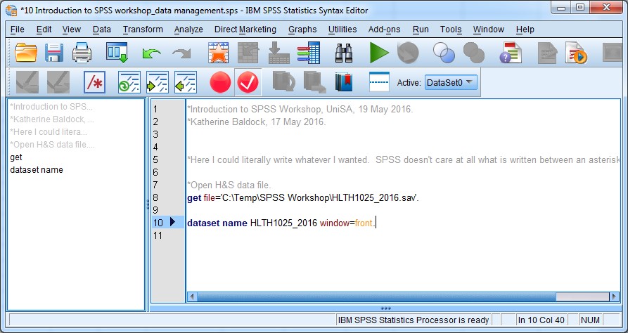
If you were wondering, the window=front code tells SPSS to make the dataset the top window (in front of everything else already open on your desktop). Notice also that I re-wrote the syntax commands in lowercase just to show you that it still works (!).
Task: Open an SPSS data file using syntax
- Save the dataset and syntax file you have open in SPSS (don’t worry about the Output file).
- Close SPSS (all files).
- Open Windows Explorer and navigate to the folder where you have saved your SPSS workshop files.
- Locate the syntax file you just created and saved, and open it by double clicking the file.
- Select all of the text in the syntax file (text and commands) and then click the “Run Selection” button on the menu bar:
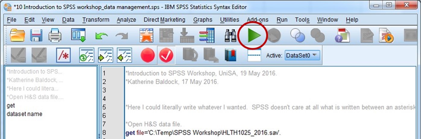
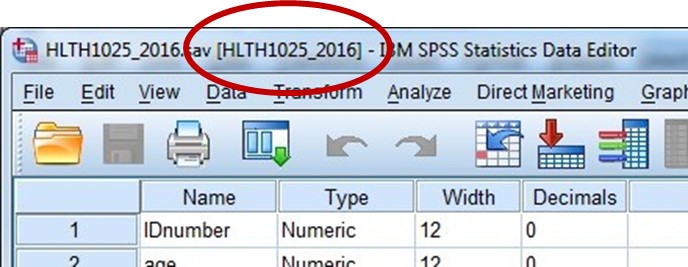
This should now open the Health and Society dataset, and label it as “HLTH1025_2016”. You’ll see the dataset name in the top right hand corner of the Data Editor window in square brackets:
Now that you know how to comment an SPSS syntax file, and can open and name a dataset using syntax, we’re going to also learn how to set a working directory (I’ll explain …) and save files using syntax.
4.2. Using syntax to ... set your working directory
![]() There’s a really neat command in SPSS (and most statistical programs have something similar) that allows you to define a directory where you are accessing and saving your files – a place like we’ve just recently set up where all our files are in the same place – called the working directory.
There’s a really neat command in SPSS (and most statistical programs have something similar) that allows you to define a directory where you are accessing and saving your files – a place like we’ve just recently set up where all our files are in the same place – called the working directory.
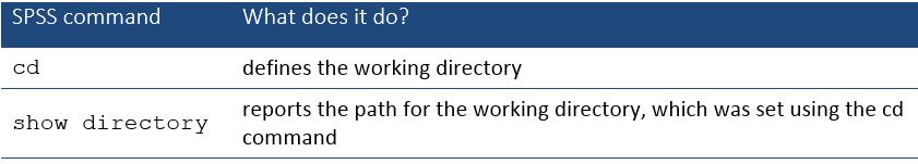
It’s good practice to define the location of your working directory at the beginning of your SPSS syntax file, and will save you a lot of time in the long run. You can do this using the cd command (cd stands for “change directory”). You can also check the working directory using the show directory command.
The key commands for defining and checking your working directory:
We are now going to define our own working directory, which will be the place you saved your SPSS files earlier. Now would be a perfect time to get out your USB stick, plug it in, and then open windows explorer to determine the file path for your working directory.
 Task: Define your working directory
- In your syntax file, under the text identifying the file, who wrote it and when it was written, but before the get file command, use the cd command to define your working folder location, e.g.,:
cd "C:\Temp\SPSS Workshop".
Notice how soon after you type “cd”, it changes colour to blue? Cool, huh?! Here’s what your syntax file might now look like:
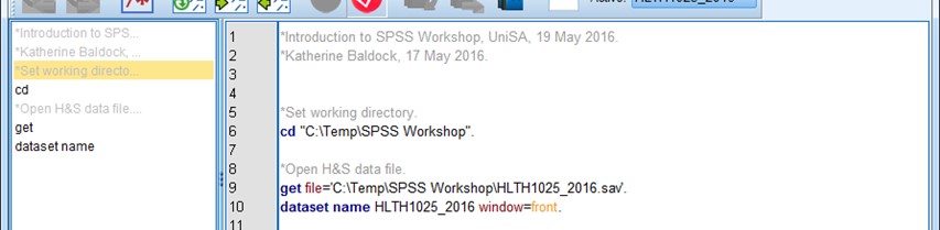
Now that we’ve set out working directory, we can modify our get file command to remove the file path (which is now set using the cd command). Now, whenever we open and/or save a file using this syntax, we won’t need to type the file path. Makes writing the syntax much easier!
4.3. Using syntax to ... save data
![]() Obviously when you create or are given a data set for your work, you need to save this file somewhere sensible. It’s really bad practice to use it from your ‘downloads’ folder, or your desktop (just for example … and yes, people actually do this … but not you!).
Obviously when you create or are given a data set for your work, you need to save this file somewhere sensible. It’s really bad practice to use it from your ‘downloads’ folder, or your desktop (just for example … and yes, people actually do this … but not you!).
The key command for saving an SPSS data file:
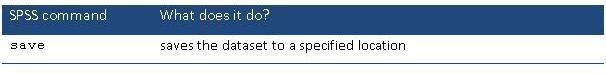
Once you’ve decided where you’re going to save your files (you would have already done this when defining your working directory, so we should be ok at this point), you can use the save command to save your file where you want it.
For those of you who are still not entirely comfortable with the concept of using/writing syntax yet, let’s first use the menus and then paste the save syntax into our open syntax file.
- Click File > Save as …
- Navigate to the working directory (where you want to save your file)
- Click Paste (right hand side of dialogue box)
- Click Yes to replacing the existing file (if that message appears…)
Your open syntax file should now have a save command, which you should comment something like this:
The thing is, though, that we’ve set the working directory already, so there’s a bit of inefficiency going on here. Also, the syntax is pretty straightforward, so let’s have a go at writing it ourselves, making use of the fact that we’ve also set the working directory up front.
 Task: Save your SPSS dataset
1. Type the following into your syntax file:
save outfile="HLTH1025_2016.sav" /compressed.
The outfile criteria tells SPSS that we want to “save out” the file to a location, which equals (=) the location we specify in quotation marks. Since we set the working directory, we now don’t need to specify the whole file path – just the file name. SPSS now knows that we want everything saved to the working directory. Efficiency!
The text at the end of the command – /compressed – tells SPSS to compress the data file to save space. This is an “option” for the save command (most commands have one or more options to be more specific about what you want SPSS to do) – options are highlighted in green.
2. Save your syntax file (CTRL + S will do the trick!).
5. Part III: Managing data in SPSS
![]() Managing data well is a really important skill, and SPSS is a good place to learn some of the basics of data management.
Managing data well is a really important skill, and SPSS is a good place to learn some of the basics of data management.
Three key elements to data management processes include:
1. Importing data into SPSS;
2. Labelling data (variables and values); and
3. Sorting and merging data.
Before and after doing each of these processes, you should also know how to inspect your data.
These four processes are covered in this chapter.
5.1. Importing data from Excel to SPSS
![]() One of the more common formats for entering and storing raw data is Microsoft Excel. If you want to work with your data in SPSS, however, you’ll need to import the data from Excel to SPSS. This can be relatively straightforward, but there are a few things to look out for in the conversion process.
One of the more common formats for entering and storing raw data is Microsoft Excel. If you want to work with your data in SPSS, however, you’ll need to import the data from Excel to SPSS. This can be relatively straightforward, but there are a few things to look out for in the conversion process.
We are going to have a go at importing a data file from Excel to SPSS, so that we can see firsthand some of the issues that may come up.
My best advice would be to make sure that you have set up your data well in Excel – this can make the importing process much easier. Also, make sure you take note of a few key data elements in your original data, such as the total number of respondents or records, and the number of variables.
 Task: Import data from Excel to SPSS
- Save all your SPSS files, and Close SPSS.
- Open the Excel file you downloaded earlier – HLTH1025_2016.xlsx
- Have a look at how the Data worksheet is set up. For instance, how many records are there? How many variables? What format are the data for each variable? If the data are numeric, make sure the format is set to “Number”.
- When you’re happy with the Excel file, Close it.
- Open your SPSS syntax file.
- Click File > Open > Data …
- Click the “Files of type:” drop down box and select Excel (.xls, .xlsx, .xlsm)
- Navigate to and select the HLTH1025_2016.xlsx file that you saved to your working directory.
- Click “Paste”, to paste the syntax to your syntax file
- A new dialogue box will appear – you should tick the box “Read variable names from first row of data”, as the H&S excel file has variable names in the first row.
- In that same dialogue box, select the “Data” worksheet to import (that’s where the data are stored).
- Click OK. This will paste the syntax to import the data – it hasn’t imported the data yet!
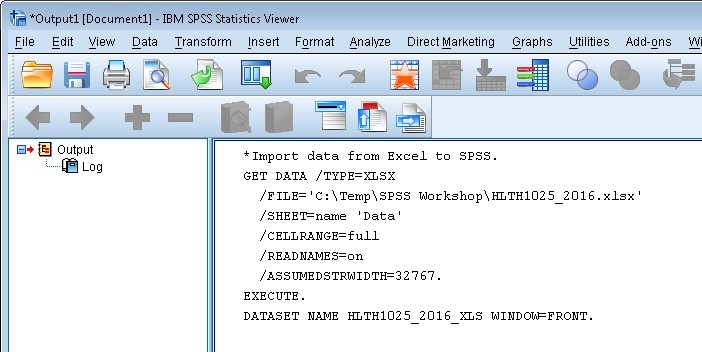
If you have a look at the import syntax, you can see that it’s doing exactly what we told it to do. Similar to the get file command, the get data command also gives you the option to name your dataset.
Select only the get data procedure and click the Run Selection button on the menu bar (the green arrow).
The first thing you should do after importing data from another format is to check your output file to see if there are any error messages. The output file is where you will see whether the syntax you have run has ‘worked’ properly.
In this case, you should not see any error messages, as in the image below:
Also, if you haven’t already put a description (comment) in front of your import syntax, you should do it now!
The next thing to do is to check that the data look like they should, e.g., numeric data has imported as numeric, string data as string, the values look ok, you have the right number of records, the right number of variables, etc. This part requires knowing how to inspect your data in SPSS, which leads us nicely into the next part of this workshop.
5.2. Inspecting your data
![]() Before you can start doing data analyses, you need to familiarise yourself with your data. I like to call this ‘getting to know your data’. There are several commands that help you to understand the characteristics your data. Some of these commands provide similar information and it’s up to you which ones you prefer to use.
Before you can start doing data analyses, you need to familiarise yourself with your data. I like to call this ‘getting to know your data’. There are several commands that help you to understand the characteristics your data. Some of these commands provide similar information and it’s up to you which ones you prefer to use.
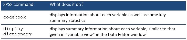
There are a couple of useful commands for inspecting your data:
 Task: Inspect your data
- The codebook command is best run through the menus if you have a large number of variables and you want to look at information for all of them
- Click Analyze > Reports > Codebook…
- Select all of the variables you want information for, and move them from the left hand box to the right hand box:
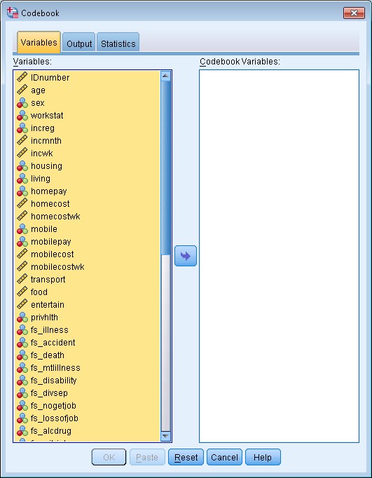
3. Click Paste.
4. Select and run your codebook syntax from your syntax file.
5. Have a look at the information presented about your variables in the Output window:
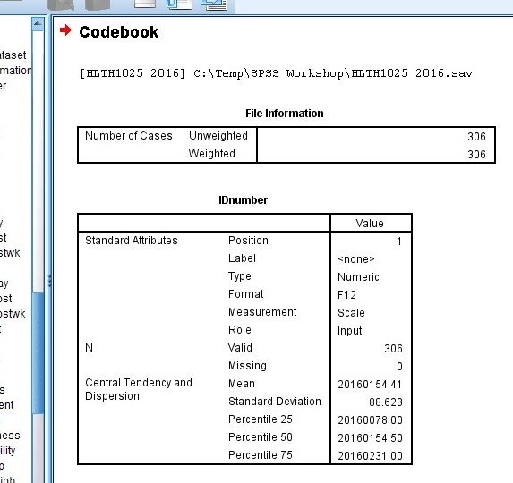
2. To display the data dictionary, all you need to type into your syntax file is:
display dictionary.
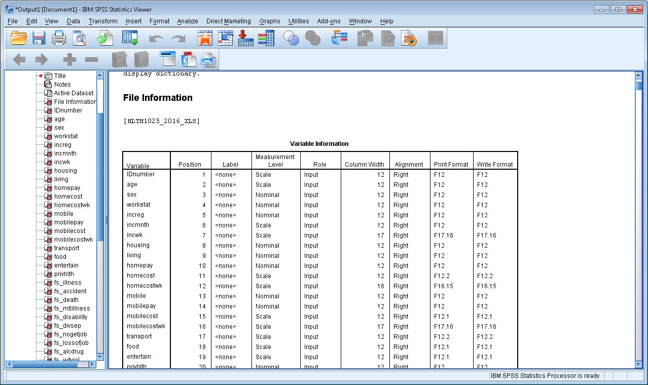
You should now see something like this in your Output Viewer window:
This is a relatively simple merge
5.3. Labelling your data
![]() Later on, when you’re running some analyses and you want to look at, say, how many of your respondents are male or female, you’ll run a procedure and the results will be displayed in the Output Viewer window. If we left our data as they are, we’d get the results we want, but we probably wouldn’t know how to read them. E.g., if I ran that procedure, here’s the output I’d get:
Later on, when you’re running some analyses and you want to look at, say, how many of your respondents are male or female, you’ll run a procedure and the results will be displayed in the Output Viewer window. If we left our data as they are, we’d get the results we want, but we probably wouldn’t know how to read them. E.g., if I ran that procedure, here’s the output I’d get:
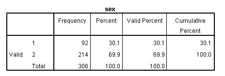
But which ones are male and which ones are female?! Because I haven’t labelled my data, it can be difficult to remember what all the values for each variable refer to.
So here’s a tip: always label your variables and their values (particularly for categorical variables).
 Task: Label variable and values for sex.
The syntax to label variables and values is pretty straightforward.
To give the variable sex a descriptive label, here’s what you could type in your syntax file:
variable labels sex Sex of respondent.
Then, to label the categories of sex (in this case, male and female), we could type the following:
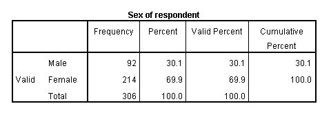
value labels sex 1 ‘Male’ 2 ‘Female’.
After labelling my variable, sex, if I run the same procedure as above I get a table that very clearly indicates what is being presented:
5.4. Sorting and merging data
![]() The sort syntax is quite simple, and you can write this yourself. If I want to sort cases by sex, in ascending order (although for this type of variable it probably doesn’t matter whether ascending or descending), I can simply type into my syntax file the following:
The sort syntax is quite simple, and you can write this yourself. If I want to sort cases by sex, in ascending order (although for this type of variable it probably doesn’t matter whether ascending or descending), I can simply type into my syntax file the following:
sort cases by sex(A).
The command to sort your data is sort cases. The “A” in brackets at the end of the statement indicates we want the data sorted in ascending order – you can write “D” if you want descending.
Let’s say now, we have an additional variable – year – that we have in a separate dataset. This second dataset has the same participants as our HLTH1025_2016 dataset, and they are identified by the variable IDnumber. But we have several years’ worth of data from this course, and when we put it all together, we want to be able to identify which students belong to which cohort (year of study).
The students we have information about belong to the second year of the study. We need to merge this variable in to our main dataset.
This is a relatively simple merge procedure, but demonstrates the key steps involved.
 Task: Sort and merge data
1. You already have open the main dataset (HLTH1025_2016). You now need to open the second dataset, called HLTH1025_2016_yr. Do this using the get file syntax:
get file=‘HLTH1025_2016_yr’.
We also want to name this second dataset – it will help us to tell SPSS exactly which dataset we want to do things with … we’ll see in a minute when we sort. So use the dataset name syntax to name your new dataset:
dataset name HLTH1025_2016_yr window=front.
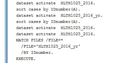
2. Now we need to sort cases by IDnumber in both datasets. Here’s where it’s helpful to have datasets named, since we can ‘activate’ a dataset to run a procedure, then activate another dataset to run the same or different procedure. It’s easy to activate a particular dataset if you’ve named it. Use the following syntax:
dataset activate HLTH1025_2016.
sort cases by IDnumber(A).
dataset activate HLTH1025_2016_yr.
sort cases by IDnumber(A).
3. Now that you’ve written the syntax to open, name and sort your data, you will need to select those lines of code and Run Selection (big green arrow button).
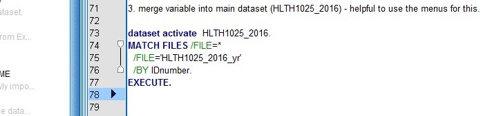
4. The final step is to merge the year variable into your main dataset. Here we are going to use the menus to help us, and then paste the syntax and run it from our syntax file.
a. First, activate your main dataset (HLTH1025_2016):
dataset activate HLTH1025_2016.
b. Click Data > Merge Files > Add Variables …
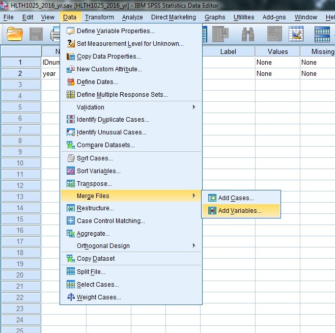 .
.
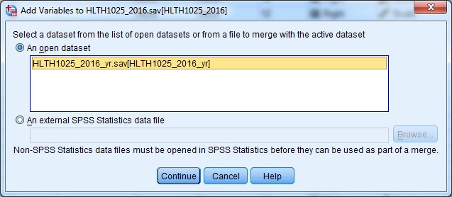
c. Select the dataset HLTH1025_2016_yr to merge with your active dataset, and click Continue:
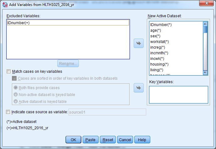
d. A new dialogue box will appear, like this:
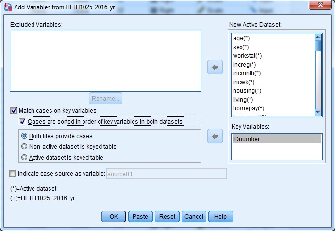
e. Tick the “Match cases on key variables” check box, and then tick the “Cases are sorted in order of key variables in both datasets” check box.
f. Click the IDnumber variable in the “Excluded Variables:” box to the top left, and move it using the arrow button into the “Key Variables:” box.
This tells SPSS to match cases in both datasets by the IDnumber variable, and we confirm that the data in both datasets are sorted by IDnumber (the variable we want to match on).
g. The dialogue box should now look something like this:
h. Click Paste to paste the merge syntax to your syntax file.
When you click Paste (or OK) a warning message will come up to say that if your data are not sorted in ascending order of the Key Variable(s) then the procedure will fail. Luckily we already sorted the data as required, so we click OK.
i. Your syntax should look something like this:
j. Select the syntax and Run Selection.
After you run a procedure like merging, it’s best to check a few things. First, I always check my output to see whether there were any error messages. Hopefully you don’t receive any error messages, and your output record looks something like this:
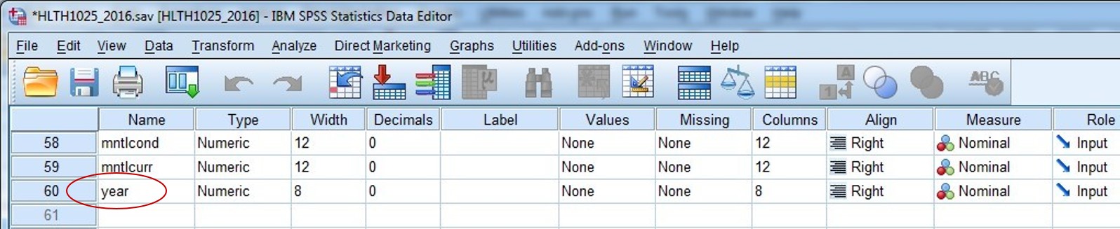
The next thing I normally check is the Data Editor window in Variable View, to see whether my new variable is now at the bottom of my list of variables, and check whether it looks like it merged correctly.
Looks good to me:
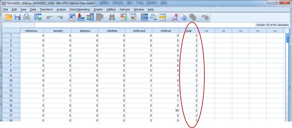
Then, I’d just double check using Data View that the values have actually merged for that variable, and that they look right. I know that all records should have a value of “2” for the variable year.
Again, it looks good:
You should now feel relatively comfortable with the sorting and merging procedures in SPSS.
6. Part IV: Describing your data
![]() Before initiating data analyses, it’s a good idea to check the frequencies of all variables, how categorical variables have been coded, the minimum and maximum values and number of missing observations. This is a good way to identify any outliers and potential mistakes in the dataset.
Before initiating data analyses, it’s a good idea to check the frequencies of all variables, how categorical variables have been coded, the minimum and maximum values and number of missing observations. This is a good way to identify any outliers and potential mistakes in the dataset.
There are several commands available to describe your data:
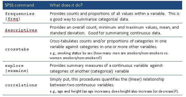
6.1. Procedures: Frequencies and Descriptives
![]() The commands frequencies and descriptives I tend to write myself in my syntax file, but I will often use the menus for crosstabs, explore and correlations, depending on what options I want to use. Regardless of whether I use syntax or menus, I ALWAYS paste the code into my syntax file so that I have a record of what I have done!!
The commands frequencies and descriptives I tend to write myself in my syntax file, but I will often use the menus for crosstabs, explore and correlations, depending on what options I want to use. Regardless of whether I use syntax or menus, I ALWAYS paste the code into my syntax file so that I have a record of what I have done!!
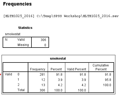
See the following for an example of the frequencies (you can shorten this to freq) and descriptives syntax:
freq smokestat.
Here’s the output:
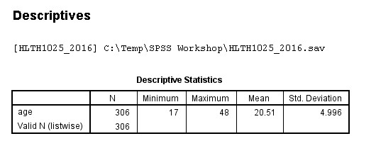
descriptives age. [total count (n), min, max, mean & SD for age]
Here’s the output:
6.2. Procedure: Crosstabs (and chi-square)
![]() Let’s cross-tabulate smoking status and sex:
Let’s cross-tabulate smoking status and sex:
1. Analyze > Descriptive Statistics > Crosstabs …
2. In the dialogue box that pops up, place your outcome of interest (smoking) in the columns, and the variable you want to group participants by (to compare one against the other) in the rows (i.e., sex):
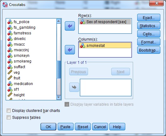
3. If we leave it at this, we’ll just get a count of respondents in each combination of categories (e.g., males who smoke, or females who are ex-smokers). But we want to know how to also get a percentage for each group. For this, we need to select the “Cells…” button to the top right of the dialogue box:
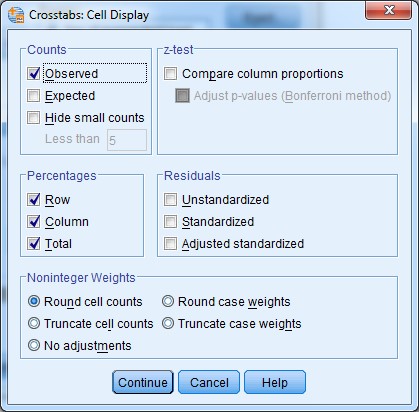
4. Here we can select percentages for rows, columns and total. Let’s select all three then click Continue, then Paste, to paste the syntax to our syntax file for the record.
5. Run selection, then look at your output:
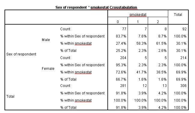
Here we can see it might be useful to label our smoking status value labels, but I can tell you that 0 = Never smoked, 1 = current smoker, and 2 = ex-smoker.
So we can see that in this cohort:
- the majority of males and females (83.7% and 95.3%, respectively) have never smoked;
- a greater proportion of females (95.3%) than males (83.7%) have never smoked;
- a greater percentage of males (7.6%) than females (2.3%) are current smokers; and
- a greater percentage of males (8.7%) are ex-smokers compared to females (2.3%).
It’s also possible to run chi square tests using crosstabs to test whether those differences observed are statistically significant. We can do this through the “Statistics…” option in the crosstabs dialogue box:
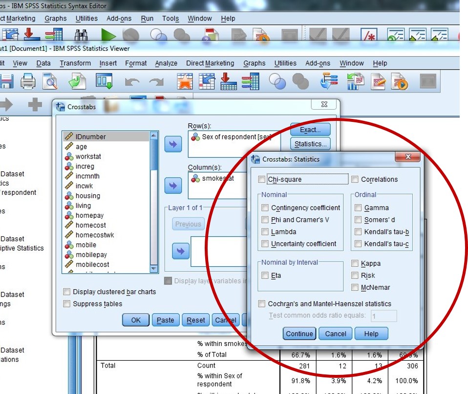
- Tick the “Chi-square” check box at the top left of the Statistics dialogue box, then click Continue.
- Paste your updated crosstabs syntax to your syntax file (don’t delete the previous one!), and run selection.
- In addition to the crosstabs results table you had before, your output should also include another table at the bottom with the results of the chi-square test:
|
Chi-Square Tests |
|||
|
|
Value |
df |
Asymp. Sig. (2-sided) |
|
Pearson Chi-Square |
11.633a |
2 |
.003 |
|
Likelihood Ratio |
10.547 |
2 |
.005 |
|
Linear-by-Linear Association |
10.714 |
1 |
.001 |
|
N of Valid Cases |
306 |
|
|
|
a. 2 cells (33.3%) have expected count less than 5. The minimum expected count is 3.61. |
|||
The Pearson Chi-spare test (top row of data in the table) indicates that there are significant differences between groups, given by the p-value less than 0.05 in the third column of the table.
6.3. Procedure: Explore
![]() As an example, let’s have a look at the mean age by smoking status categories.
As an example, let’s have a look at the mean age by smoking status categories.
- Analyze > Descriptive Statistics > Explore …
- Place your categorical variable (smokestat) in the “Factor List:” box, and your continuous variable (age) in the “Dependent List:” box.
- Click Paste, then run selection from your syntax file.
- Your output should look something like this:
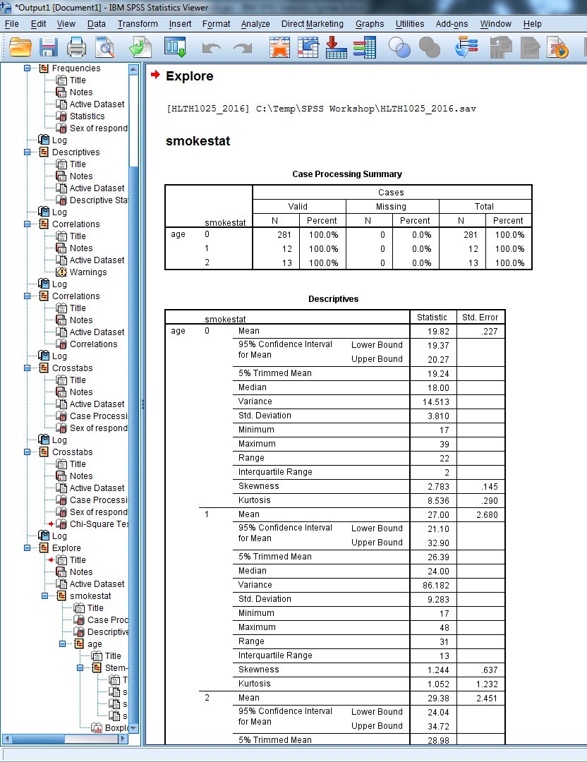
This tells us, for example, that the mean age of those who have never smoked, is 19.8 years (SD=3.8), and that the mean age for current smokers is 21.1 years (SD=9.3). You can see that we also get a lot of other descriptive information about age according to smoking status.
6.4. Procedure: Correlations
![]() For our final descriptive procedure, we’ll have a look at the correlation between weight and height.
For our final descriptive procedure, we’ll have a look at the correlation between weight and height.
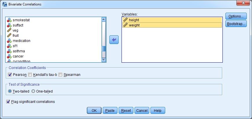
1. Analyze > Correlate > Bivariate …
2. All you need to do is add the two continuous variables of interest (weight and height) into the “Variables:” box, and click Paste.
3. Run selection in your syntax file and then look at your output:
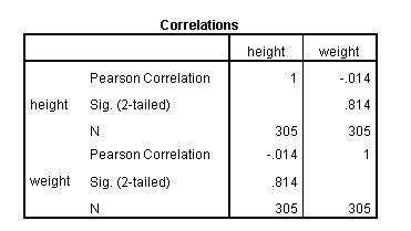
4. This table gives us the results of our procedure. It tells us that there is a weak, negative association between height and weight of -0.014, and that it is not statistically significant (p>0.05).
7. Part V: Modifying your data
![]() Normally when we collect data, we don’t get everything in the format that we actually want to analyse. For example, in a survey we often collect information about height and weight – but what we really want to know is their body mass index (BMI). We use the height and weight data to calculate this, and create a new variable BMI. We might then also want to categorise our new BMI variable into: underweight, normal weight, overweight & obese.
Normally when we collect data, we don’t get everything in the format that we actually want to analyse. For example, in a survey we often collect information about height and weight – but what we really want to know is their body mass index (BMI). We use the height and weight data to calculate this, and create a new variable BMI. We might then also want to categorise our new BMI variable into: underweight, normal weight, overweight & obese.
We’re now going to look at a couple of very commonly used commands to modify, and create new variables from, existing data.
Key commands to modify your data:
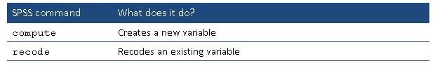
You can access these procedures from the menus, under the Transform menu. There are many things you can do here, such as create standardised variables (with a mean of 0, SD of 1), create new variables from ntiles (tertiles, quartiles, quintiles, deciles, etc.), and many more. It’s worth having a look to see what you can do.
The compute and recode commands can be used for simple data modification processes, though, so we’ll write the code ourselves in our syntax file.
7.1. Compute a new variable
![]() First, let’s compute a new variable, BMI, from weight and height [Note: BMI = weight/height2]:
First, let’s compute a new variable, BMI, from weight and height [Note: BMI = weight/height2]:
1. Compute a new variable, heightm (height in metres)
compute heightm=height/100.
execute.
2. We should check our newly created variable heightm – how should we do this?
3. Compute another new variable, BMI:
compute bmi=weight/height**2.
execute.
[Note: exponentiations are denoted as ** in SPSS]
4. Check your new variable, BMI – how ??
7.2. Recode an existing variable into a new variable
![]() Now that we have our new variable BMI, we want to recode it into a new variable, bmicat, where the BMI values are categorised into underweight (BMI<18.5), normal weight (BMI >=18.5 and <25), overweight (BMI >=25 and <30), and obese (BMI>=30).
Now that we have our new variable BMI, we want to recode it into a new variable, bmicat, where the BMI values are categorised into underweight (BMI<18.5), normal weight (BMI >=18.5 and <25), overweight (BMI >=25 and <30), and obese (BMI>=30).
Here is the code to write in your syntax:
recode bmi (sysmis=sysmis) (lowest thru 18.499999=1) (18.5 thru 24.99999=2) (25.0 thru 29.99999=3)
(30 thru Highest=4) into bmicat.
execute.
The recode command is followed by the variable name (bmi), then we put in brackets the value ranges for each category, and give them a label (1, 2, 3, and 4 for the four categories). We also tell SPSS that any data that were missing (sysmis) we want to be missing in our new recoded variable. We are recoding the bmi variable INTO a new variable, bmicat.
If we didn’t include the “into bmicat” at the end of the syntax, we would recode the original bmi variable and would lose the individual BMI values and replace them with categories. I like to keep my original variables, so tend to use the INTO option to recode into a new variable.
8. Getting help
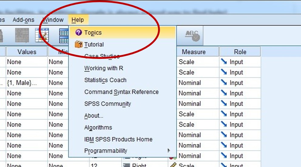
![]() SPSS has well-developed help facilities. In addition, Google is always a good way to find help! Within the SPSS interface, there are two options for getting help:
SPSS has well-developed help facilities. In addition, Google is always a good way to find help! Within the SPSS interface, there are two options for getting help:
1) Help > Topics; and
2) Help > Tutorial:
Also see the online IBM SPSS knowledge centre, which is like a searchable manual for SPSS: https://www.ibm.com/support/knowledgecenter/SSLVMB/welcome
There are also some other excellent online resources, such as this SPSS Tutorials website: http://www.spss-tutorials.com/
9. References
![]() IBM 2016, IBM Knowledge Center: SPSS Statistics, IBM, viewed 18 May 2016, <https://www.ibm.com/support/knowledgecenter/SSLVMB/welcome/>.
IBM 2016, IBM Knowledge Center: SPSS Statistics, IBM, viewed 18 May 2016, <https://www.ibm.com/support/knowledgecenter/SSLVMB/welcome/>.
van den Berg RG 2013, 8.1.1 SPSS Syntax – Six reasons you should use it, SPSS Tutorials, viewed 17 May 2016, <http://www.spss-tutorials.com/spss-syntax-six-reasons-you-should-use-it/>.
van den Berg RG 2015, 1.2.1 SPSS Combining data with syntax and output, SPSS Tutorials, viewed 17 May 2016, < http://www.spss-tutorials.com/spss-combining-data-with-syntax-and-output/>.
van den Berg RG 2016, SPSS Tutorials, viewed 17 May 2016, <http://www.spss-tutorials.com/>.