Descriptive data analysis: COUNT, SUM, AVERAGE, and other calculations
| Site: | learnonline |
| Course: | Research Methodologies and Statistics |
| Book: | Descriptive data analysis: COUNT, SUM, AVERAGE, and other calculations |
| Printed by: | Guest user |
| Date: | Tuesday, 19 May 2026, 3:13 PM |
Description
This tutorial will give you the opportunity to consolidate some key skills in data management and descriptive data analysis that you will use in ALL of the assessments for this course.
Table of contents
- 1. Introduction
- 2. What is Excel?
- 3. Opening and saving your dataset
- 4. Orientation to the 1025 Study dataset (Excel Workbook)
- 5. The =AVERAGE function
- 6. The =STDEV function
- 7. The =COUNTIF function
- 8. The =SUM function
- 9. Write your own formula: Calculate a Proportion (%)
- 10. Create a graph in Excel
- 11. Time to Practice!
1. Introduction
Part 1 of this Excel module will introduce you to the structure and format of an Excel file, and we will learn how to undertake some basic descriptive analyses of health data. We will be using the software program Excel to manage our data, undertake a few key calculations, and present the data in a graph.
This first part of the Excel module will give you the foundational skills to help you in subsequent parts of the module.
On completion of Excel module: Part 1, you should be able to:
1: Navigate an Excel data sheet by identifying the data contained in rows versus columns;
2: Calculate means, standard deviations, counts and proportions using formulas in Excel; and
3: Create a graph in Excel.
2. What is Excel?
Excel is a software program which is a standard part of Microsoft Office (just like Word and PowerPoint). All computers in the UniSA computer pools have Microsoft Office installed.
Introductory Activity
Locate and open Excel on the computer you are currently using. When you open Excel for the first time, you will see a spreadsheet.
On top of the spreadsheet (just like in Word), there is a menu and icons.
At the bottom is a "tab" or worksheet which is named “Sheet 1". Next to this there is a little "plus" sign in a circle. If you click on the "plus" sign it will add another worksheet - you can have a go! If you right click on any of the worksheet tabs you can rename it.
Excel files are essentially books made up of one or many worksheets.
Excel is a very useful program and once you feel comfortable with it, you should be able to find MANY uses for this throughout your studies and in your future career.
Ok ... so now you know what a blank/new Excel workbook looks like…you are ready to move on!
3. Opening and saving your dataset
For this introductory module in Excel, we are going to use data from a student cohort who were enrolled in a population health course in 2015 at UniSA and who form part of a study, the 1025 Study.
Here, we're just going to download and save the 1025 Study 2015 dataset.
Tasks:
1: Right click on the file below to save a copy of the 1025 Study, 2015 dataset (in Excel format). You should select the "save as ..." option, and save the file to your USB drive:
![]() 1025 Cohort, 2015 dataset (.xlsx format, 95 KB)
1025 Cohort, 2015 dataset (.xlsx format, 95 KB)
2: Open your saved copy of the dataset. It should look something like this:
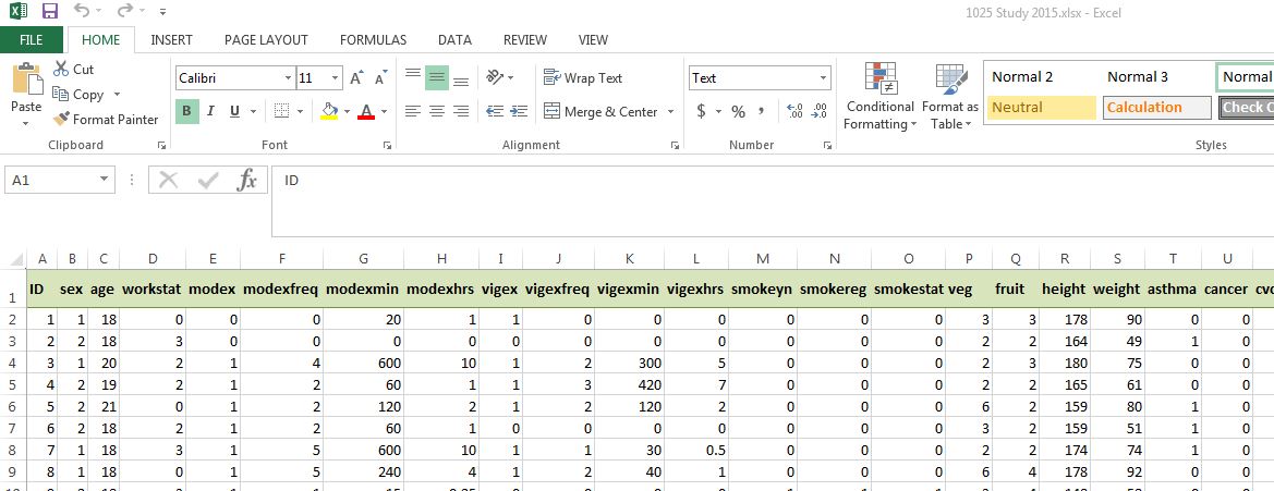
You may notice that the spreadsheet doesn't quite look the same as a blank spreadsheet (coloured headings, borders, etc). This spreadsheet has been formatted to make it easier to find where you need to be in the spreadsheet.
[Note: Learning how to format spreadsheets (and documents in general) to make information easier for someone to read/grasp, is an important skill, so I'd encourage you to have a go at trying out your own formatting as you go through this module.]
4. Orientation to the 1025 Study dataset (Excel Workbook)
Key concepts:
-
Cells make up the rows and columns in the spreadsheet. Cells generally hold a single piece of information. -
Rows represent individuals (cases): each row contains one individual's (case's) responses to each survey item (question). -
Columns represent survey items (questions), which we call "variables". -
An Excel "workbook" (file) is made up of one or more "worksheets". -
Metadata is information about data sets (e.g., where did the data come from) and the data contained within them (e.g., what each variable represents and how it is coded in the data set).
For those of you who are not yet comfortable with numeric data ... this is an example of a dataset with text data instead of numeric data:
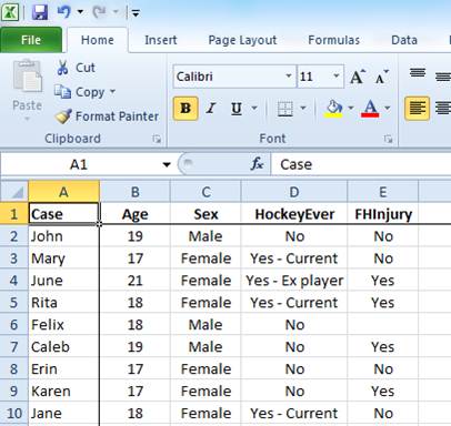
In this dataset, we are looking at a survey of people with regard to their participation in the sport of Hockey, and whether they've had an injury as a result of the sport. It contains information about participant names, ages, sex, whether they have ever played hockey (no, yes I'm an ex-player, yes I'm a current player), and whether they've ever had an injury.
This is straightforward enough, but we can't do any calculations on it, because the data is (mostly) in text format. I can't calculate a count of people who have ever played hockey, nor determine the proportion of males versus females in my survey. To do these things, I need to store this information as numeric data and assign values to response options.
While it can be daunting to look at an unfamiliar dataset for the first time (or first few times!), once you understand what the data represents it will become less scary!
In the "Data" sheet in the 1025 Study dataset, identify the variables (columns) that represent age, sex and height.
Using these variables, we are going to calculate the following :
- mean (average) age of the 1025 Study 2015 cohort and the standard deviation (SD);
- count (number, or 'n'), total count, and proportion (%) of males and females; and the
- mean (average) height and standard deviation (SD) of the student cohort.
5. The =AVERAGE function
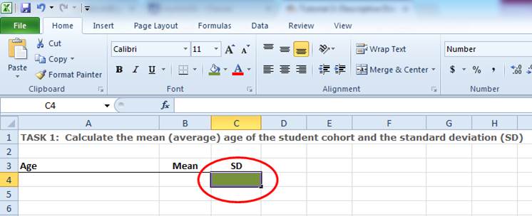
1: Calculate the mean age of your student cohort
The first calculation is a mean (also called an average). In Excel, the 'formula' we need to use to tell Excel to calculate a mean looks like this:
=average([cell range])
The cell range we enter in this formula is the column of data (variable) for which we want to know the average or mean value.
We are going to learn how to use the formula bar to do our calculations.
STEPS:
-
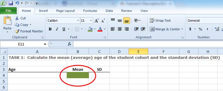
- In your "calculations" worksheet, locate the appropriate cell to enter the mean age for your cohort and select it (click on the cell) with your mouse. You should see a dark border now around the cell:
-
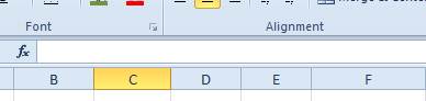
- While the cell is still selected, click on the empty white part of the formula bar:
-
- Type the following (the beginning of a formula) into the formula bar:
=average(
-
- Click on the "Data" worksheet down the bottom left of the screen
- With your mouse, select the data range (column of data) for the variable age (e.g., cells B2:B32)
- Press the Enter key on your keyboard - this completes the formula by adding a closing bracket at the end of the formula.
You have now calculated the mean age of your student cohort. Before doing anything else, SAVE your workbook!
Did you all get the same answer?
TIME TO PRACTICE:
Following the same process as above, calculate the mean height of your student cohort.
How did you go?
6. The =STDEV function
2: Calculate the standard deviation for the mean age of your student cohort
- In your "calculations" worksheet, locate the appropriate cell to enter the SD for the mean age of your cohort:
- While this cell is selected, type the following into the formula bar:
=stdev(
- Click on the "Data" worksheet down the bottom left of the screen
- With your mouse, select the data range (column of data) for the variable age (e.g., cells B2:B32)
- Press the Enter key on your keyboard to complete the formula (alternatively you can click back into the formula bar and type ")" at the end)
You have now calculated the standard deviation for the mean age of your student cohort. Now SAVE your workbook!
Did you all get the same answer?
TIME TO PRACTICE:
Following the same process as above, calculate the SD for the mean height of your student cohort.
How did you go?
7. The =COUNTIF function
3: Calculate the count of students in your cohort by sex
- In your "metadata" sheet, find the numeric value that corresponds to being male
- In your "calculations" worksheet, locate the appropriate cell to enter the count of students who are male:
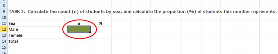
- With your mouse, select the cell in which you want to enter the count of students who are male.
- In the formula bar, type the following:
=countif(
- Click on the "Data" worksheet down the bottom left of the screen
- With your mouse, select the data range (column of data) for the variable sex (e.g., cells C2:C32)
- Type the following into the formula bar:
,1)
This will complete the formula: =countif([cell range],[criteria for being male])
- Press the Enter key on your keyboard
You have now calculated the count of males within your student cohort. Now SAVE your workbook!
Did you all get the same answer?
TIME TO PRACTICE:
Follow the same instructions as above to calculate the count of students in your cohort who are female.
(HINT: Remember to check your "metadata" worksheet to find the numeric value that corresponds to being female to use in the formula)
How did you go?
8. The =SUM function
In order to calculate a proportion (the next section in this tutorial), you will need to have calculated the total count (sum) of students with valid data in your student cohort.
5: Calculate the total number (sum) of students in your cohort with valid data for the variable sex
- In your "calculations" worksheet, locate the appropriate cell to enter the total number (sum) of students who have entered data for the variable sex:
- With your mouse, select the cell in which you want to enter the total number of students.
- Type the following into the formula bar:
=sum(
- With your mouse, select the data range (column of data) for the n (count) of males and females (i.e., cell range B20:B21).
- Press the Enter key on your keyboard to complete the formula.
You have now calculated the total count (sum) of males and females within your student cohort. Now SAVE your workbook!
Did you all get the same answer?
9. Write your own formula: Calculate a Proportion (%)
4: Calculate the proportion (%) of students in your cohort who are male
- In your "calculations" worksheet, locate the appropriate cell to enter the proportion of students who are male:
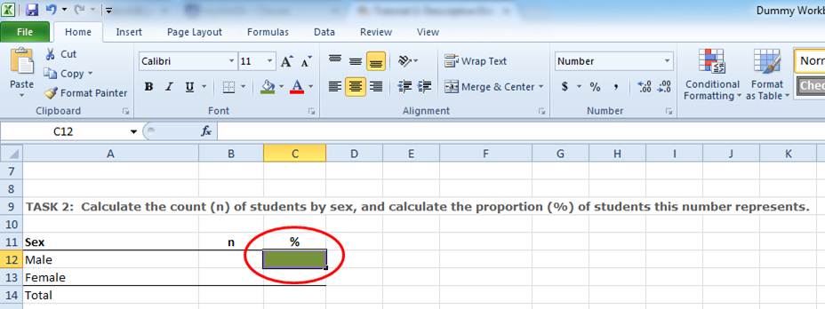
- With your mouse, select the cell in which you want to enter the proportion of students who are male.
- You will need to now calculate the following formula:
=([count of males] ÷ [total n of students])
NOTE: In Excel, "divide by" (÷) is represented using the character "/".
You can enter these counts/totals manually, or you can select the cell in which they are located as follows:
1. In the formula bar, type:
=
click in the cell containing the count of males
this cell reference (e.g., C27) should now be written in the formula bar after the equals sign (=)
3. click back into the formula bar and type:
/
4. click in the cell containing the total count of students
5. click back into the formula bar and finish the bracket:
)
- Press the Enter key on your keyboard
You have now calculated the proportion of males within your student cohort.
BUT ... often we like to present proportions as percentages (%). To do this we need to multiply the proportion by 100. Adding this to the original formula would look like this:
=([count of males] ÷ [total n of students]) x 100
NOTE: In Excel, "multiply by" (x) is represented using the character "*".
- Select the cell with the proportion of males in the student cohort
- In the formula bar, click at the end of the existing formula, and type:
*100
- Press the Enter key on your keyboard
You have now calculated the proportion (%) of males in your student cohort.
Now SAVE your workbook!
Did you all get the same answer?
TIME TO PRACTICE:
Using the same process as above, calculate the proportion of females within your student cohort.
How did you go?
10. Create a graph in Excel
In this section, we are going to walk through how to create a graph in Excel using the calculations for sex that you performed in the previous section.
STEPS:
1. In your "Calculations" worksheet, select the entire table with the data you have calculated for sex. Copy this table (either click the "copy" button in the top left hand corner of your "Home" menu, or right-click where you have selected the table and click "copy").
2. Open your "Graph" worksheet, and paste the table you have just copied in an appropriate place (e.g., underneath the main heading for the worksheet).
To paste the table so that it contains the numbers you want, not the formulas, you will need to right-click where you want to paste your table, and select "Paste values" (the option with the picture "123") from the "Paste Options" section.
3. Using your mouse, select the data labels including the title cell for the sex categories (males and females).
4. While those cells are still selected, hold down the ctrl key and select the data range including the title cell for the proportions in each sex category.
5. Making sure the two cell ranges are still selected, click the "Insert" menu at the top of the Excel window, select the "Column" chart type > 2D (first option).
This will automatically insert a column graph (chart) into the "Graph" worksheet.
Charts have several key components that you will need to modify or format:
- chart title
- axis titles
- axis labels
- data points (data series)
- legend
You can find the menus for formatting graphs here:
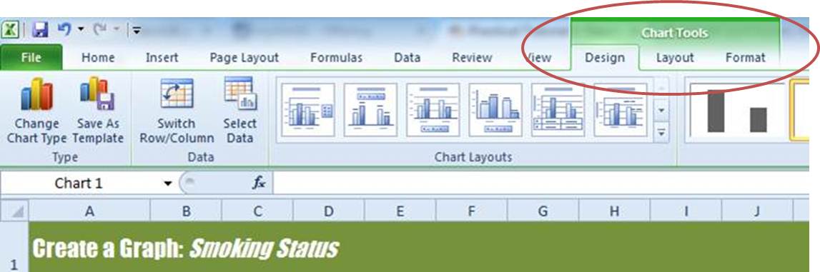
6. Spend the next 10 minutes or so having a go at changing/modifying each of these chart components on the chart you just created.
11. Time to Practice!
Now it's time for you to have a go at practicing what you've just learnt using different variables.
Using the instructions from the previous sections, calculate the following:
- count (n) and proportion (%) of each category of diabetes status; and the
- mean (average) weight of your student cohort and the standard deviation (SD)
Go to Part 2: COUNTIFS function