Practical 3: Friction and Minor Losses in Pipes
| Site: | learnonline |
| Course: | Introduction to Water Engineering |
| Book: | Practical 3: Friction and Minor Losses in Pipes |
| Printed by: | Guest user |
| Date: | Tuesday, 26 May 2026, 3:24 PM |
Description
Practical 3: Friction and Minor Losses in Pipes
Introduction
The energy required to push water through a pipeline is dissipated as friction pressure loss, in m.
“Major” losses occur due to friction within a pipe, and “minor” losses occur at a change of section, valve, bend or other interruption. In this practical you will investigate the impact of major and minor losses on water flow in pipes.
Major losses

Minor losses

where
f = friction factor
k = minor loss coefficient
L = Length (m)
D = Diameter (m)
V = Velocity (m/s)
Supporting Information
Major Losses
Pressure loss is proportional to L/D ratio and velocity head. For low velocities, where the flow is laminar, friction loss is caused by viscous shearing between streamlines near the wall of the pipe and the friction factor (f) is well defined.
For high velocities where the flow is fully turbulent, friction loss is caused by water particles coming into contact with irregularities in the surface of the pipe and friction factor itself is a function of surface roughness.
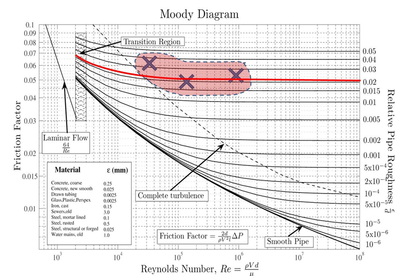
In most engineering applications, the velocity is less than that required for fully turbulent flow and f is a function of both the viscosity of a boundary layer and the roughness of the pipe surface. Values of f can be determined experimentally and plotted in dimensionless form against Reynolds Number Re to from a Moody Diagram.
Minor Losses
Minor losses behave similarly to major losses, where a device with a large k value leads to a high pressure loss. In general, a very sudden change to the flow path contributes to significant pressure loss.
Apparatus
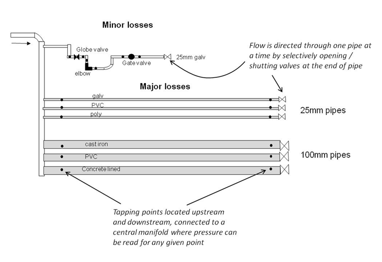
Five materials are available for investigating friction losses:
- Concrete lined (100mm)
- Cast iron (100mm)
- P.V.C. (100mm & 25mm)
- Galvanised iron (25mm)
- Polyethylene (25mm)
Surface roughness will be calculated from observed pressure loss at a given flow rate.
Pressure tappings in the pipes are connected to the pressure gauge for indication of pressure reading.
A 25 mm galvanised iron line contains a set of valves and bends for investigating minor losses.
Gallery
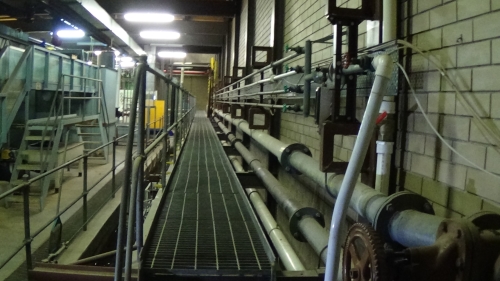
Different types of pipes create different amounts of friction thereby impacting on the flow rate.
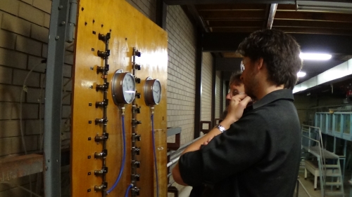
The changes in water pressure, through the different pipe types, is measured at the end of the rig.
Experimental Method

Slides and notes as PDF (502KB)
- Select a pipe and pass a high speed flow through it. Record flow and pressure readings. The pressure loss between upstream and centre, and centre and downstream tapping points must be taken separately. Reduce the flow in stages, taking readings of pressure loss and flow rate
- Repeat for all pipes
- Establish one flow rate in the minor losses line and record pressure levels across each device. Note that a length of pipe between tapping points also contributes to the observed pressure loss.
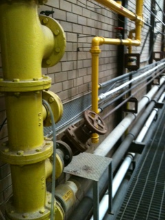
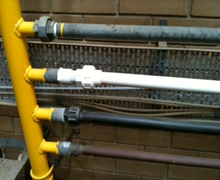
The image above is of the friction loss experimental rig showing the different pipes travelling off of the main yellow down pipe.
Data for Analysis
Please download this excel spreadsheet to obtain data for this experiment.
You will see that for the major losses, each pipe had three different flow rates passed through it. In each case, the pressure was measured upstream and downstream to determine the overall pressure head loss over the length of the pipe. You will use this to determine the Darcy friction factor, and in turn use the friction factor to determine the relative roughness of the pipe (k/D).
For the minor losses, a single flow rate was passed through the pipe and the pressure was measured upstream and downstream of several typical objects (two valves and an elbow bend). These were all in 25mm galvanised steel pipe. It is important to note that the observed pressure head loss in these cases is due to both the minor loss in the object itself and a small amount of pipe friction. For this reason, you have also been given the length of pipe between the two measurements. You will need to use an appropriate friction factor from your analysis of 25mm galvanised steel pipe in the first part of the experiment (major losses).
Calculations
For all of the calculations in this practical you will need to convert the pressure difference into a head measured in metres:
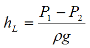
Where P1 and P2 are respectively the upstream and downstream pressure in Pascals.
Major Losses
You will be using the observed head loss hf to determine the friction factor λ and hence the relative roughness (k/D) for each pipe. Then you will compare the absolute roughness (k) with typical roughness values for each pipe material (you can find such values in textbooks or on the internet).
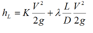
We’re assuming that the entire pressure difference is due to friction in the pipe. So the observed hf can also be given by the Darcy equation:
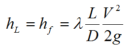
As you know hf, L, D and V (which you can get from the flow rate and diameter using the continuity equation), you can rearrange this equation for the friction factor λ. For each pipe, three flow rates were passed through the system so you will need to perform the calculation three times to get three different values of λ.
To obtain the relative roughness (k/D) you also need the Reynolds number (Re):
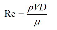
You can assume the dynamic viscosity (μ) is 1.005 x 10⁻³ kg/ms.
Now you have two options to obtain k/D. One is to plot the values of λ and Re on the Moody diagram above.
Once you have plotted your three points on the Moody diagram, you can estimate an “average” curve (see the red line in the example diagram) that follows the same basic shape as the other curves on the chart. (Note that it is very common in this experiment for results to be spread out such that the average curve does not pass neatly through all three points. In these cases you could also plot an upper and lower curve to capture the “spread” of the results.) The point where your average curve exits the chart on the right is where you can infer the value of relative roughness. If you have plotted an upper and lower curve to capture a wide spread of results, you can infer an upper and lower value of k/D accordingly.
The alternate method is to rearrange the Moody equation to determine k/D. The Moody equation is used to generate the lines on the Moody diagram so you will get a more accurate result by using the equation directly. The equation is as follows:
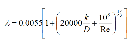
It is straightforward to rearrange this to obtain k/D in terms of Re and λ.
Minor losses
In the case of the minor losses, the observed head loss is due to the loss in the object itself plus pipe friction:
You have been given the length between the two tapping points, the flow rate and the observed pressure difference (which you convert to hL). The minor loss experiment was conducted in 25mm galvanised steel pipe, which means you have can determine velocity.
You will need to refer to your calculations from the Major Losses part of the experiment in order to determine an appropriate value for λ. You can either calculate λ using the Moody equation (or diagram) from the k/D value you obtained earlier for galvanised steel, or, if the velocity in the minor loss experiment is quite close to one of the velocities used in the major loss experiment (for 25mm galvanised steel) you might simply use the value of λ from that experiment.
Once you have a value for λ, the only unknown in the equation is the head loss coefficient K. You can therefore determine a value of K for each object and compare these against typical values for each device (you can find published values in textbooks or on the internet).