> Exercise: Introducing the Symbolic Toolbox

> Type in the following commands.

clear all

sin(x)

>What error message is displayed?

> Type in the following and see if you still get the same error message.

syms x

sin(x)

The syms command is actually a shortcut for the sym command. The longer way of writing is:

sym(‘x’)

> Exercise: Symbolic Variables

> Type in the following and decide which variables are symbolic.

syms x

y = x + 1.4*sqrt(x+3) + 5.49

pretty(y)

>What does the pretty command do here?

> Exercise: Using solve for a Single Equation

> Go through and type in the code for the following steps to solve the single equation.

$\frac{10}{x^{3}+1} =4-2x$

> Watch out! There is an error that you will need to correct!!

In this case

$f(x)= \frac{10}{x^{3}+1} -4+2x$

> Exercise: Another Example of Solving Symbolic Equation

> Solve the general quadratic equation $ax^{2}+bx+c=0$ for any x by making the three coefficients $a, b, c$ and $x$ symbolic variables.

syms a b c x

> Instead of creating a new variable f for function, use the following command to solve directly:

soln = solve(a*x^2+b*x+c)

The above command doesn’t specify the variable to solve for. If it is not specified, the solve command will:

1) Solve for x by default or

2) Solve for the last alphabetical variable if there is no variable called x or

> Exercise

> Solve the equation again, replacing $a$ with $u$, $b$ with $v$, $c$ with $w$ and $x$ with $s$.

syms u v w s

...

> What is the answer this time?

> Exercise: Using solve for Simultaneous Equations

> Use MATLAB to find the solution of the following simultaneous equations:

$2y+3x=4$

$5y-2x=5$

> This time you will need to create two functions, f1 and f2 to solve f1=0 and f2=0 using the following command:

[x,y] = solve(f1,f2)

> Exercise: Using the ezplot command

> Type the following code and examine output plots.

syms x

ezplot(sin(x))

ezplot(sin(x),[-pi pi])

hold on

ezplot(sin(x))

ezplot(3*x+2)

hold off

• array of $x$- coordinates
• array of $y$- coordinates

• function handle
• endpoints

• symbolic function
• endpoints

• does not need a function formula
• full control of graph parameters

• function is stored in M-file for easy access (via handle) and modification

• can easily create a graph using only two lines of code

• requires more code to generate

• must create a function M-file if it is not MATLAB in-build function

• function is not stored in easily accessible M-file,
• graphs have the same colour

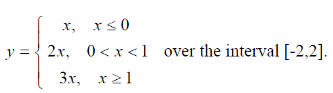
Example:

Create a graph of the function

Which plot command would you use?

Answer:

The answer depends on your overall task.

If you will need this function for further calculations, then use fplot command. To use fplot, you will need to create a function M-file, specifying the three parts of the function separately by using if statements.

If you want just to plot this function, then use ezplot with hold on and hold off commands to plot it ‘piece-by-piece’, specifying endpoints.

clear all

syms x

hold on

ezplot(x,[-2, 0])

ezplot(2*x,[0, 1])

ezplot(3*x,[1, 2])

axis([-2 2 -2 6])            %why do you need to do this?

title(‘Piece-wise function’) %what changes will happen if you delete this command?

hold off

Note: If you plot several functions using ezplot, then the title of the figure will be of the last function plotted. The hardest option for this sort of function is to use the plot command. Otherwise, all the above options are relatively same.

Quickly check that the equation $speed=20ln(t+1)$ accurately reflects the speed of a car for $t$ between 0 and 10 seconds.

Hint: use ezplot.

> Exercise: Graphing

> In the table below you are given the results of a student’s weekly assignments to plot.

> Which graphing technique would you use in this case?

> Exercise: Evaluating Equations

Consider the function $f(x)=\left(x^{3}+2\right) \sec x$

> Define this function $f$ in the Symbolic Toolbox, by first defining $x$ as a symbolic variable.

> Find $f(0.157)$  by evaluating this function at $x = 0.157$ using the subs command as follows:

y = subs(f,x,0.157)

> Find $f(0.123)$ by evaluating this function at $x=0.123$ using the eval command as follows:

x = 0.123

y = eval(f)

As you can see the difference in these two examples is only in the number of commands you need to use to evaluate the function at a certain $x$.

> Exercise: Variables’ substitution

> Type the following commands, where function $f$ is the same as in the previous example.

syms t

y2=subs(f,x,t)     %substitutes x with t

y3=subs(f,x,t-1)    %substitutes x with t-1

y3=simple(y3)       %to simplify the expression for y3

> Exercise: subs Command

> Define function $f(x)=x^{4}-5x^{2}+4$ in the Symbolic Toolbox. Make sure that you typed syms x before the function’ definition. Substitute $x$ with $\sqrt{t}$ using subs command. Do not forget to type syms t before substitution.

> Exercise: Numbers

> Use the polynomial roots command to find the roots of the polynomial $p \left(x\right)=x^{2}+9x+6$

> Now, define $x$ as a symbolic variable and define the polynomial $p$ in MATLAB as follows:

p = x^2+9*x+6

> Use the solve(p) command to find the roots using the Symbolic Toolbox.

> What is the difference between the answers for the standard and symbolic methods?

> Exercise: Using Algebraic Operations

> Let $p(x)=x^{2} \left(x+4\right)^{2}-8x \left(x+1\right)^{2}+13x-6$

> Define $p$ in a script M-file called symPoly.m using the following commands:

syms x

p = x^2*(x+4)^2-8*x*(x+1)^2+13*x-6

> Now use the algebraic operations to help you create the following five cells.

1. Expand p
2. Find the factors of p
3. Store the coefficient array of p in a variable called coeff_p
4. Use the solve command to find when p = 0
5. Now try the polynomial roots command together with double to find the roots of $p(x)$ in standard MATLAB format.

> Exercise: Finding Derivatives & Integrals

> Open your script M-file symPoly.m with the equation $p \left(x\right)=x^{2} \left(x+4\right)^{2}-8x \left(x+1\right)^{2}+13x-6$.

> Create two new cells using the following commands to find the 1^st and 2^nd derivatives of $p(x)$ as well as the indefinite and the definite integral from -1 to 1.

dp=diff(p,x)                 % note that you do not need to specify x because it is the default variable

d2p = diff(p,x,2)            % How would you find the third derivative of x?

intp = int(p,x)

intpDef=int(p,x,-1,1)

> Exercise: Limitations of Integration Techniques

> Create a symbolic equation  $f \left(v\right)= \frac{ \sin v}{v+e^{v}}$

> Use the int command to find the indefinite integral, and observe the output.

intf = int(f,v)

> Modify the above command to find the definite integral between v=0 and v=pi.

Does the command work?

> Observe what happens if you use the double command.

defint=double(int(f,v,0,pi))

x=a

eval(f)

Definite integral of $f(x)$ with endpoints $a$ , $b$