6. Function M-files
Almost all of the MATLAB commands that you have been using are stored in function M-files. Before fully explaining the construction of this type of M-file, it is worth looking more deeply inside MATLAB to view some of them.
1. The MATLAB type command enables you to view the content of any M-file, including the many hundreds stored inside the MATLAB software. After the prompt, enter type(’cos’). The response is merely “cos is a built-in function” and so no documentation is available as to how MATLAB actually evaluates cos(x).
2. However, now enter type(’gammainc’). The M-file gammainc.m, located in Specialized Math Functions, contains a special function, namely the Incomplete Gamma Function = γ(x, a). You do not need to be familiar with this function. Examine the first line
function b = gammainc(x,a)
The first word function is essential and indicates this is a function-type M-file. gammainc is the name of the function and must correspond to the name of the M-file, gammainc.m.
There are two input variables, namely x (which could be a scalar or an array) and a (which is usually a scalar). There is one output variable b which is the same length as x.
Now go to the end of the M-file gammainc.m. You will notice that the output variable b is finally given a value.
To see this function working, after the >> prompt enter gammainc(4,1.5) (ans=0.9540) and gammainc([3 3.5 4],2.28) (ans= 0.7427 0.8189 0.8745). Note that the input and output variables x,a,b are dummy variables merely used to define the function.
3. Enter type(’linspace’) after the prompt. This displays the content of linspace.m, in Elementary Matrices and Matrix Manipulation, which is the function M-file containing the linspace command. The first line is
function y = linspace(d1,d2,n)
You are aware that the input dummy variables d1,d2 are the ends of the interval and n is the number of points. Notice that the only executable commands in this M-file are
if nargin = = 2
n = 100;
end
y = [d1+(0:n-2)*(d2-d1)/(n-1) d2];
The first three lines set n=100 by default if you forget to input a value for n. The last line determines the output array y containing the n points. Exercise: check that this formula is correct.
4. Enter type(’quadL’) to view quadL.m in Function Functions - Nonlinear Numerical Methods. This function finds a numerical approximation to
where funfcn(x) is any function, either built-in by MATLAB or defined by you in a function M-file funfcn.m as explained in the next Section 6. The first line is
function [Q,fcnt] = quadl(@funfcn,a,b,tol,trace,varargin)
The last three input variables are optional. The ouput variable Q contains a value for the integral, while fcnt is optional if you require extra information. At the end of this M-file notice that values are calculated for these output variables. (Do not bother looking at all the commands in between.)
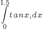
Exercise: Enter quadL(@tan,0,1.5) to show that an accurate estimate of

