6. Function M-files
Constructing
Why might you wish to define and construct your own functions and store them in function M-files?
- the mathematical formulation of a function might be quite long and complicated. It might be better to define it separately rather than inside a script M-file.
- the same expression of one or more variables might be required a number of times, either within a single M-file or on different occasions. It is more economical to define the expression as a function in an M-file.
- many MATLAB commands operate on functions which must be held in function Mfiles (see Section 6).
Once a function has been constructed by you in an M-file, it can be used in the same ways as all other MATLAB functions. It can be evaluated, used in any other M-file, or differentiated/integrated in the Symbolic Math Toolbox (see Section 8). In fact, your function can later be used in constructing yet another new function.
The first time MATLAB executes a function M-file, it opens the file and compiles the commands into an internal representation in memory that speeds their execution for all ensuing function calls.
Suppose you wish to construct a function myfunc. Function M-files must follow specific rules.
- The function name and the M-file name must be identical. Therefore, a function myfunc must be stored in a file named myfunc.m.
- The first executable statement must be of the form function
output_variables = myfunc(input_variables) - Do not include any clear commands inside a function M-file.
- Each executable command most probably will finish with a semicolon to avoid printing out numbers each time the function is accessed. Any required values can be printed in the Command Window or in the calling script M-file.
- Each output variable should be given a value within the M-file.
- Function M-files terminate execution and return output values when they reach the end of the M-file, or if they encounter the command return beforehand.
Note: You cannot run a function M-file by entering the name of the M-file after the >> prompt as you do with a script M-file. You must give values for the input variables and evaluate as an arithmetic expression.
Example 1: The number of different combinations of r items from n items is given by the binomial coefficient
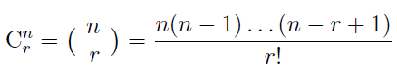
where n ≥ 1 and r ≥ 0 are integers, r ≤ n. Create a function M-file comb.m containing the function comb(n,r):
function y=comb(n,r)
if r = = 0 % no space between the two equal signs
y=1;
return
end
top=prod([n:-1:n-r+1]);
bottom=prod([1:r]);
y=top/bottom;
Now enter after the prompt
comb(4,0) , comb(3,3) , comb(5,2) , comb(9,5) , comb(25,14)
Example 2: Consider the function
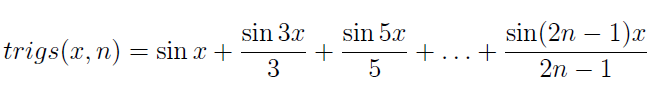
where x is the point (or array of points) where the function is being evaluated and n is the number of terms used in this series of sine functions. For example,
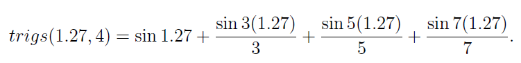
Construct the function M-file trigs.m:
function y=trigs(x,n)
% commence the sum for y with the first term
y=sin(x); % y is an array if x is an array
for k=2:n
kodd=2*k-1;
y=y+sin(kodd*x)/kodd;
end
Now evaluate trigs(1.27, 4) (=0.8347) and trigs(1.27, 40) (=0.7822).
You can, of course, now plot a graph of trigs(x, n) for a given n. Construct the following script M-file and then run it.
clear all
x=linspace(-2*pi,2*pi,801);
y=trigs(x,4);
axis([-2*pi 2*pi -1 1])
hold on
plot(x,y)
hold off
Change the trigs(x,4) to each of trigs(x,40) and trigs(x,200) and execute. The graphs you see are part of Fourier Series theory.