This is really a fancy name for asking what a typical value of the variable is. For example, what is a typical weight of the students? In common language, we call a measure of central tendency an average. However, in statistics there is more than one measure of central tendency or average. The most commonly used ones are the arithmetic mean (often just called the mean) and the median. You may occasionally come across the mode, which is the most common frequency - for example, in the student weights data set, the mode was 50-59 kg. However, because the mode is very difficult to handle mathematically, we tend to not use it much.

The Mean

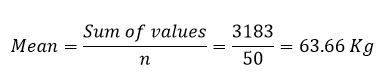
The mean is the most commonly used measure of central tendency or typical value. It is very easy to handle mathematically, simple to calculate, and usually falls in the middle of the data set. To calculate the mean, we simply add up all of the values and divide by the sample size. For our student weights:

In statistics, we often use shorthand to make the formula easier (at least for statisticians) to read. For example, instead of “Sum of values” we use the Greek letter sigma (Σ). Thus you might find the above formula written in a textbook as:

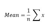
where x represents the variable to be summed.

Let us now return to the histogram and the shape of distributions. Have a look again at Figure 2. Imagine if you can, instead of having 10 kg categories for weight we had 1 kg categories, and a sample size of 1,000. Now imagine if we had 1 gm categories and a sample size of 100,000. As the category size gets smaller and smaller, and the sample size gets bigger and bigger, the number of bars in Figure 1 would get greater and greater, and the outline would change from a ragged shape to a beautiful smooth curve. Eventually, it might look like the shape you see in Figure 3. This distribution shape is known as the Normal or Gaussian distribution, and is very commonly found in variables related to health.

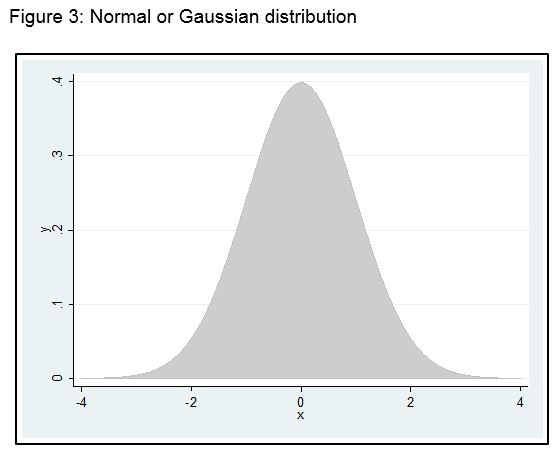
Note that if a variable has a Normal distribution, the mean, median (and mode) all fall in exactly the same place, the centre of the distribution. Variables that tend to have a Normal distribution are those that have lots of inputs going into them. For example, blood pressure can be impacted on by age, weight, obesity, genetics, sex, position of the body etc.

The Median

However, some variables we measure in health do not have a symmetrical distribution. These are typically variables with only a few inputs. Blood lead levels in children is a good example. The two key factors driving blood levels in children are the child’s age (blood lead peaks at about 12 months) and exposure to a source of lead. Because of this, the distribution of children’s blood lead levels is asymmetrical, or in statistics, we say it is skewed. In the case of blood lead, it is skewed to the right positively skewed. This is because most children have very low levels of blood lead, but some (for example those living near a smelter), have very high levels.

When the variable of interest has a skewed distribution, the mean is no longer a good typical value. This is because the extreme values in the long tail drag the mean towards them. This happens because of the way the mean is calculated. Instead, we use another measure of central tendency – the median. To obtain the median, we simply sort all our observations in to size order, and take the middle one. This works fine for an odd number of observations. For an even number of observations, we take midpoint between the two middle ones. Let’s have a look at the weight data sorted into size order, and provided in Table 3.

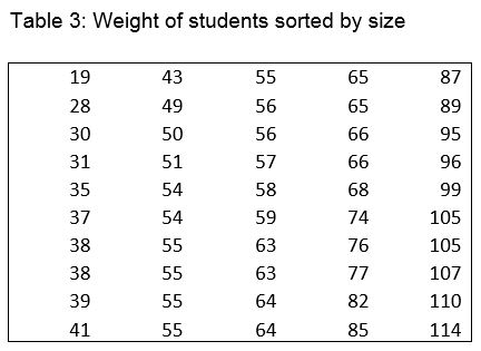
Since there are 50 observations, the median lies midway between the 25^th and 26^th observation, that is halfway between 58 and 59, so the median is 58.5.

To demonstrate a skewed distribution and its impact on the mean, I have taken the weight of the students, and deliberately changed some of the higher values to lower values. Figure 4 shows the result.

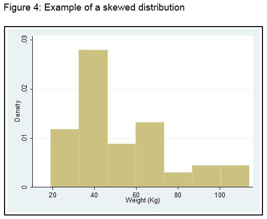
The distribution is clearly skewed with a long right hand tail, i.e., it is positively skewed. For the above data, the mean is 52.9 kg, whereas the median is 43.0 kg, clearly demonstrating that the mean is no longer a typical value for this dataset.