As well as knowing what a typical value is for a variable, we also like to know how spread-out the observations are around that typical value. In other words, are they tightly clustered around the mean, or very scattered. In order to measure this, a sensible question might be “what is the average distance of each observation from the mean?” Let’s have a look at an example. Here are some observations:

4   4   6   2   5   3

The mean of the above observations (hopefully you can calculate it in your head) is 4. To get the average distance from the mean, we subtract the mean from each observation, add up these differences, and divide by 6. Let’s have a go:

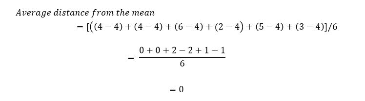
What has happened is that because some observations are greater than the mean, and some less, when you add the differences up, they always come to zero! Hmmm – so not a particularly useful measure of dispersion. To get around this problem, we square the distance of each observation from the mean. 

The Standard Deviation

The standard deviation (commonly abbreviated to sd), is the usual measure of dispersion or variability that you will see in published papers. Its formula looks complicated, but the idea is relatively straightforward. The variance is the square of the standard deviation, and we will look at how that is calculated first:

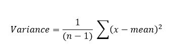
In other words, subtract the mean from each observation, square the result to get rid of the minus sign, add up all of these values, and divide by (n – 1). In the above equation, n - 1 is called the degrees of freedom (you will often see the abbreviated to df). We use (n – 1) rather than n because we already know the mean value, and this makes one observation redundant. You are probably scratching your head at this!

Suppose I told you that five numbers had a mean of 3. The numbers are:

1    5    4    2    ?

Since the mean is 3, the total must be 5 x 3 = 15. Therefore the missing number has to be 3. In other words, if you are given the mean, you only need n -1 observations to calculate the last one.

If the original observations were in kilograms, then the variance is in units of kg². To get it back to the original units, we take the square root of the variance to arrive at the standard deviation. Thus:

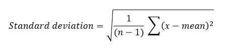
So when we are describing a set of observations with a Normal distribution shape, we present the mean and standard deviation. For our weights of 50 students shown in Table 1, the mean is 63.7, the variance 541.9 kg², and the standard deviation 23.4 kg.  As an aside, things like the mean, standard deviation, median, and proportion obtained from a sample are called sample statistics. 

The range and Interquartile range

We pointed out earlier, that the mean is not a good typical value for skewed distributions. However the formula for the standard deviation includes the mean. Does this imply that the standard deviation is not valid as a measure of variability for skewed distributions? In short, yes!

The median was calculated by first sorting all observations into size order and then taking the middle value. If we sort all observations into size order, then calculate the cumulative percentage for each observation as we go along, the cumulative percentages are known as percentiles. Table 4 shows an example of this process.

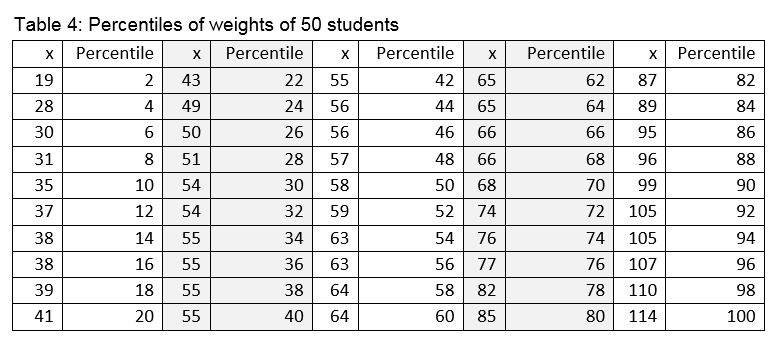
In order to describe the spread or variability of the variable when it is skewed we usually use either the range or interquartile range (IQR). The range is the difference between the maximum and minimum value. In the table above, this is 114-19 which equals 95 kg. In fact most researchers report the maximum and minimum values rather than the range. The IQR is the difference between the 25^th and 75^th percentile.  In the above table, this is 76.5-49.5 which is 27 kg.