5. Importing data into R
A data-frame is essentially the equivalent of a spreadsheet, but it is much more powerful. A dataframe is defined by columns and rows, and each column can contain different types of data much like a spreadsheet. However, a while column can contain only one type of data, there are many different formats that can be used - including lists or even a whole new dataframe! We will keep it simple for this course and just focus on numbers or letters for now.
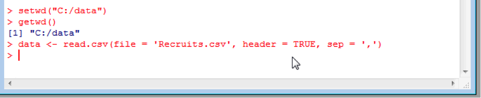
To import our data set into R, we first need to tell R where the “working directory” is. The working directory is where R will look for data and save data by default. This is done with the setwd(“<directory path>”) command. You can also check what the working directory is with the getwd() command. Please note, that file paths use forward slashes, not back slashes:
setwd(“C:/data”)
getwd()

This process also reinforces how to use functions with R, which we touched upon earlier in the list ls() function. Functions are called by name (here setwd) followed by brackets with the arguments (modifiers) to the function (here the directory path “C:/data”). Getwd is called without arguments because we just want to know what the working directory is, so the brackets are empty.
Now we tell R to import the data by creating dataframe, called eg. “data”, containing the contents of the Recruits.csv file:
data <- read.csv(file = 'Recruits.csv', header = TRUE, sep = ',', na.strings=c("",".","NA"))
The function is read.csv. The first part of the arguments (file = “ ”) says which file we wish to import. The second argument (header= TRUE) indicates whether or not the first row of the file is a set of labels (ie. column headings). The third argument (sep = ‘ ’) indicates the delimiter (in this case it's a comma as it is a .csv file). The latter two arguments are actually the default values that R would assume, and so these arguments could be left out of your command if you wish (ie. you could have just typed data <- read.csv(file = 'Recruits.csv'). However, let’s say you has a text file where the delimiter was a semi colon “;”. Then you would replace the colon with a semi colon:
data <- read.csv(file = 'Recruits.csv', header = TRUE, sep = ';')
Or perhaps there was no header line containing the column labels:
data <- read.csv(file = 'Recruits.csv', header = FALSE, sep = ',')
another useful argument is na.strings, which allows you so specify what defines a missing value. The default is no entry at all in the data (hence this argument wasn’t used above). However, people often choose to use all sorts of symbols, for example NA or a period – or worse yet, several different symbols! You can specify these yourself, for example:
data <- read.csv(file = 'Recruits.csv', header = TRUE, sep = ',', na.strings=c("",".","NA"))
If we wish to view the contents of the dataframe, we can simply type in its name as before. However, with a large dataframe this will be very long listing, and we would have to scroll a long way back to the top to see the headings. To have a quick look at the data we can use the head and tail commands to view the beginning and end of the dataframe, respectively.

Now you can see the imported data. Note that missing values are shown as “NA”. These functions have the default arguments of 6 lines of data. To modify this include the argument specifying the number of lines you want to see. For example, to see 10 lines of data, type:
head(data, 10)
If you wanted to find out more about the dataframe, for example to check how many entries there are, you can do this using the dim or str functions:

As we can see, there are 205 entries (rows) and 10 variables (columns), just like we expected when we looked at the raw data in Excel. The str function also lists the variable names, denoted with a $ sign, and gives the first few values in the data frame.