15. Test of Normality
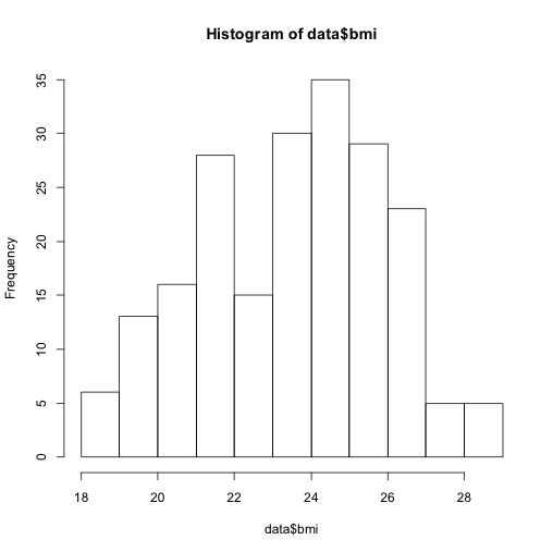
For a quick look at the shape of a distribution, try hist. For example,
hist(data$bmi)
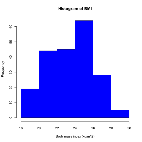
Using arguments, you can control the number of bins and colour of the plot:
hist(data$bmi, breaks=5, col="blue")
Add a proper x-axis label (xlab = “..”) and a heading (main = “..”):
hist(data$bmi, breaks=5, col="blue", xlab="Body mass index (kg/m^2)", main="Histogram of BMI")
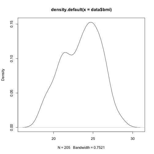
Alternatively you might like to see a density plot. First you must determine the density data, by creating an object (which I have called “dens_bmi” but you could call it what you like). Then plot the desity data.
dens_bmi <- density(data$bmi)
plot(dens_bmi)
Again, you can give the plot a better heading, and colour it:
plot(dens_bmi, main="Density distribution of BMI", col="blue")
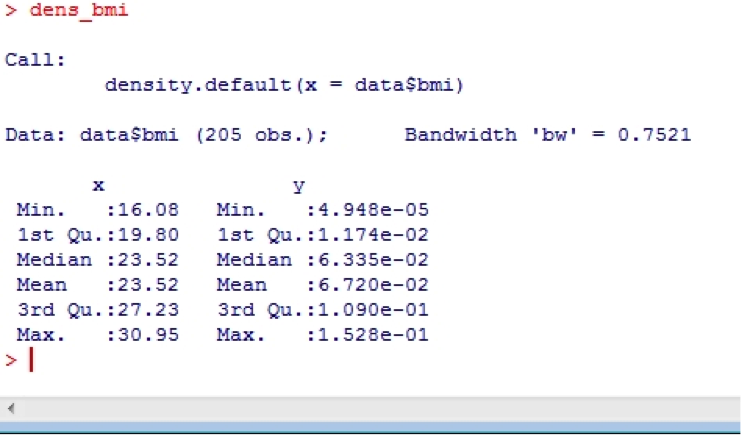
You can also ask for the density data by calling the object you just created
dens_bmi
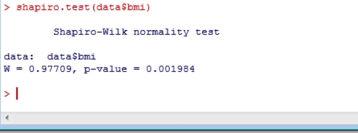
Or perhaps you’d like a more formal test? If so, you can use the Shapiro- Wilk statistic:
shapiro.test(data$bmi)