Regression is performed in R using the linear model function lm().  This can perform single and multiple linear regression analyses. Similar to the other analyses, it’s best to create an object to store the results, and then ask for a summary.  Note that we should use the factors we created earlier for boot type (bootsf) and gender (genderf).  Suppose we want to know whether age, gender and type of boots can predict boot comfort score:

fit_comfort_age_boots_gender <- lm(comfort ~ age + genderf + bootsf, data = data)

summary(fit_comfort_age_boots_gender)

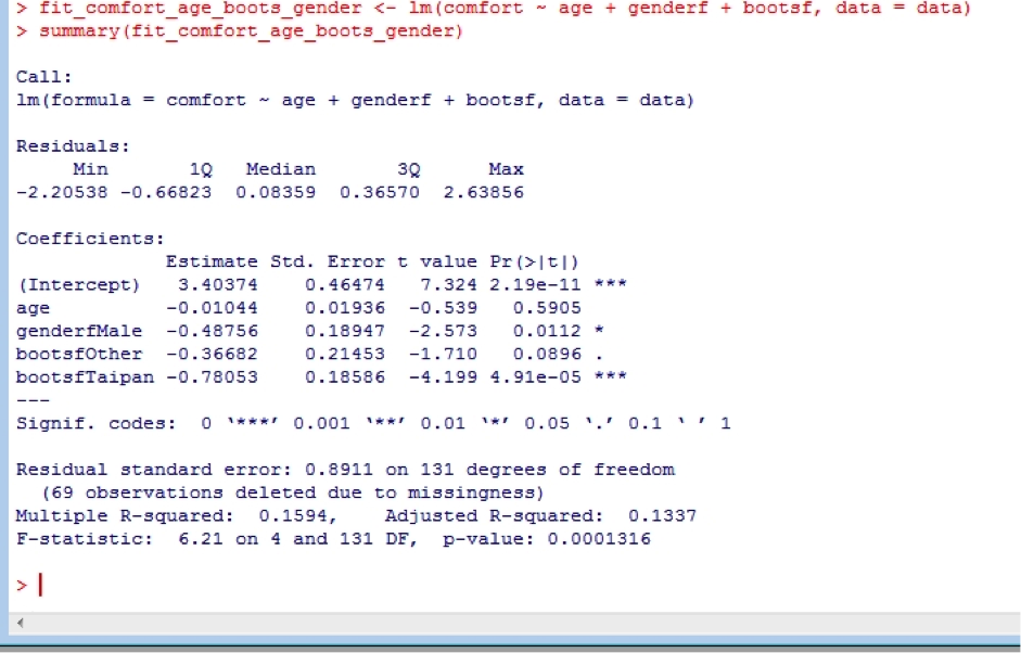
We see that overall, the type of boot worn is strongly associated with boot comfort.  Interestingly, we see that female recruits give lower comfort scores than males. This is because when this study was undertaken in about 2000, female boots were actually made from male boots lasts, and so provided a sub-optimal fit. This has now been fixed, and female recruits have their own lasts.

Other useful aspects of the analysis include:

coefficients(fit_comfort_age_boots_gender) # model coefficients

confint(fit_comfort_age_boots_gender, level=0.95) # Confidence Intervals for model parameters, here set to 95%

fitted(fit_comfort_age_boots_gender) # predicted values

residuals(fit_comfort_age_boots_gender) # residuals

anova(fit_comfort_age_boots_gender) # anova table

vcov(fit_comfort_age_boots_gender) # covariance matrix for model parameters

influence(fit_comfort_age_boots_gender) # regression diagnostics

To undertake regression diagnostics, try this:

layout(matrix(c(1,2,3,4),2,2)) # optional 4 graphs/page

plot(fit_comfort_age_boots_gender)

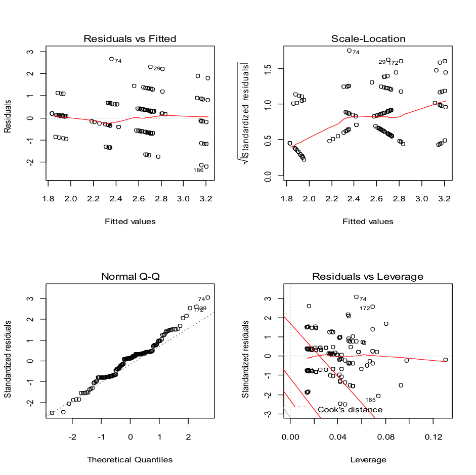
Which looks reasonable, but we can also undertake a Shapiro-Wilks test on the residuals to check if they are normally distributed. First you will need to create an object containing the residuals.  This is done using the command we used above, but making it produce and store the result as an object.  the residuals

fit_res <- residuals(fit_comfort_age_boots_gender)

shapiro.test(fit_res)

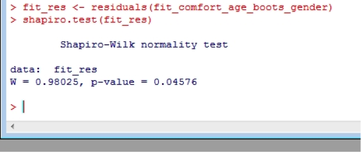
Which shows that the residuals aren’t normally distributed, but this isn’t uncommon with smaller datasets.