Special | A | B | C | D | E | F | G | H | I | J | K | L | M | N | O | P | Q | R | S | T | U | V | W | X | Y | Z | ALL
P |
|---|
PyTorch | ||
|---|---|---|
Installation instructions:
| ||
S |
|---|
Self-supervised learning | ||||||||||||
|---|---|---|---|---|---|---|---|---|---|---|---|---|
In his 2018 talk at EPFL and his AAAI 2020 keynote speech, Turing award winner Yann LeCun referred to self-supervised learning (SSL, not to be confused with Secure Socket Layer) as an algorithm that predicts any parts of its input for any observed part. A standard definition of SSL remains as of writing elusive, but it is characterised by [LZH+23, p. 857]:
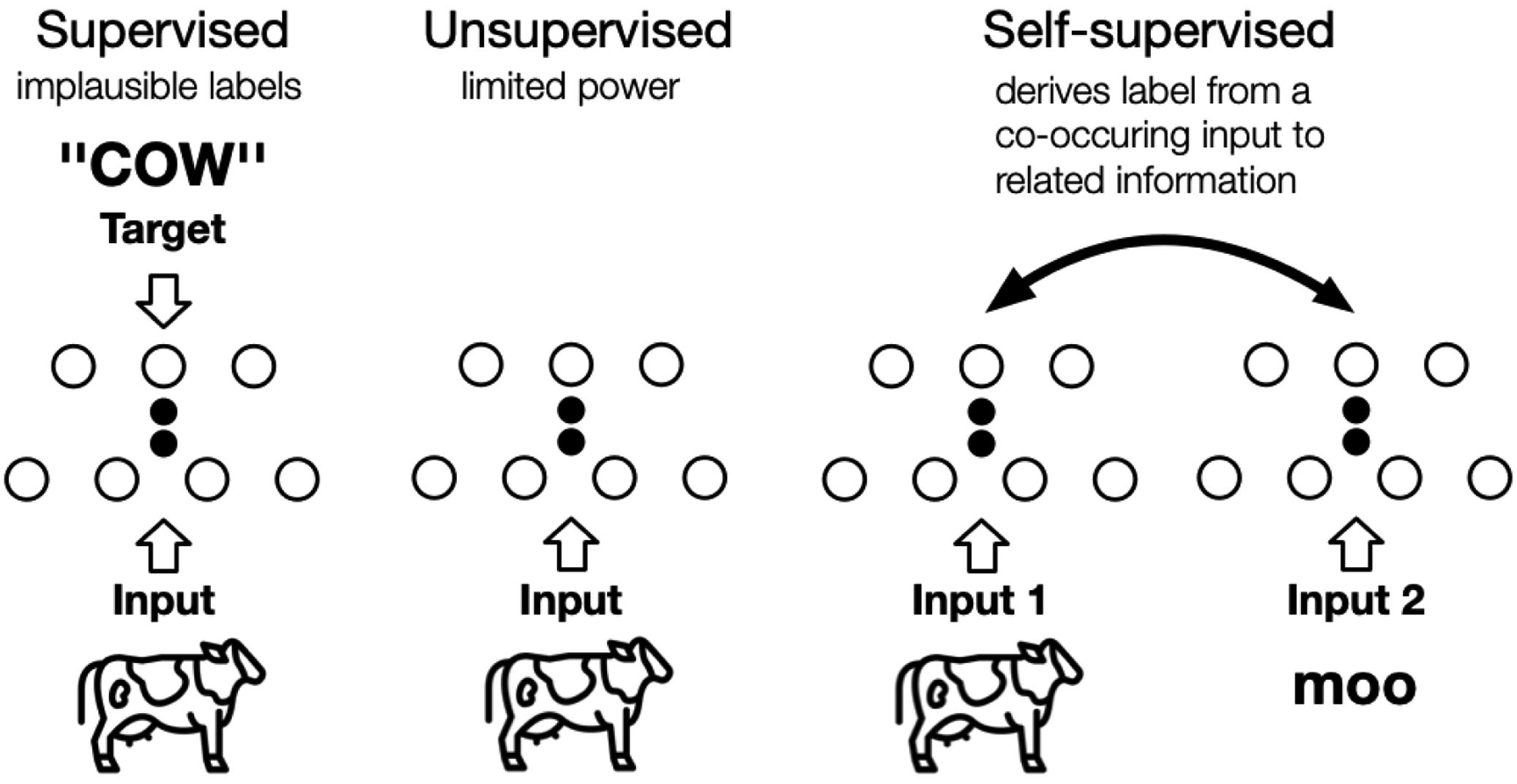 SSL can be understood as learning to recover parts or some features of the original input, hence it is also called self-supervised representation learning. SSL has two distinct phases (see Fig. 2):
 Different authors classify SSL algorithms slightly differently, but based on the pretext tasks, two distinct approaches are identifiable, namely generative and contrastive (see Fig. 2); the other approaches are either a hybrid of these two approaches, namely generative-contrastive / adversarial, or something else entirely. 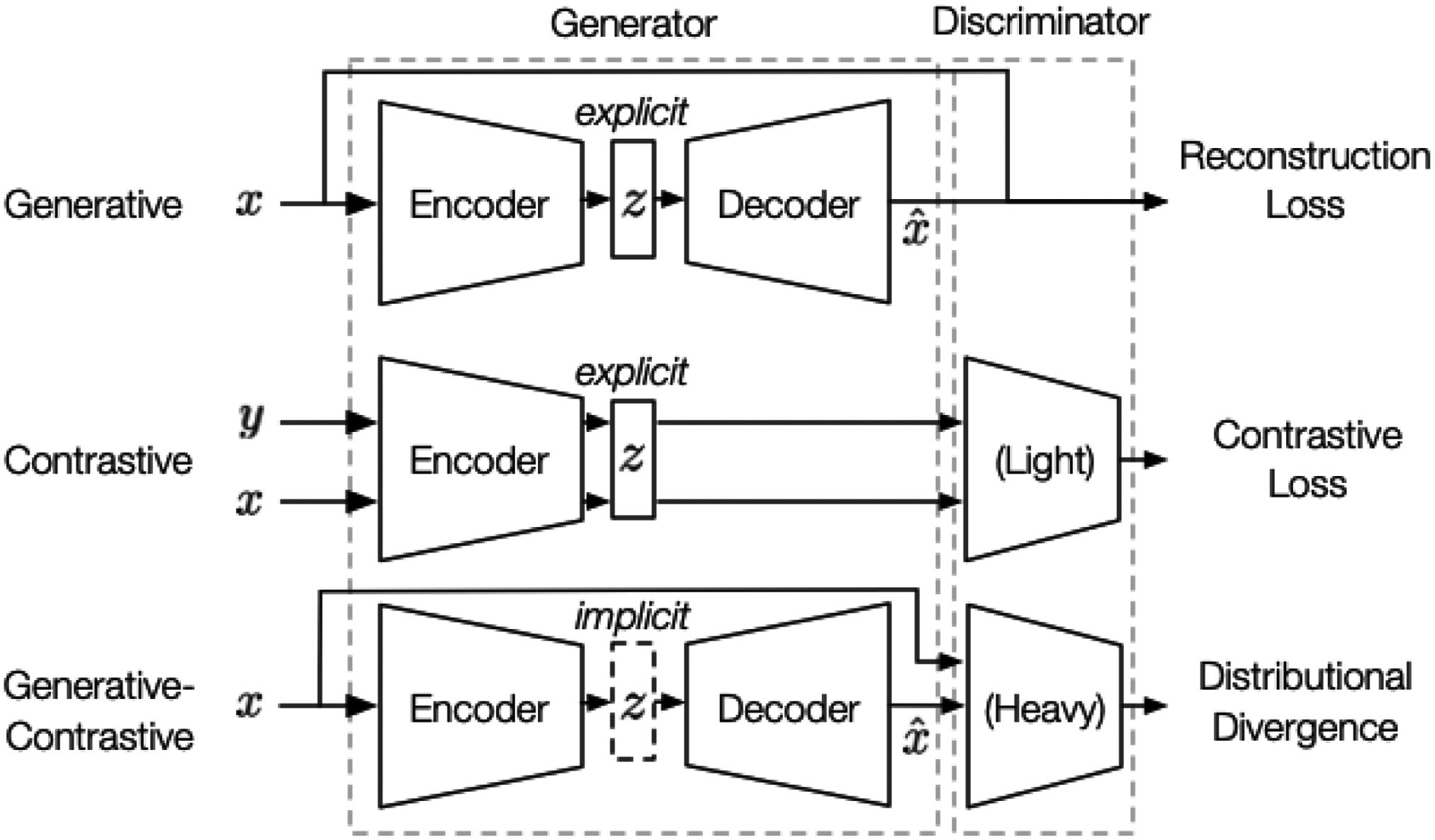 In Fig. 3, the generative (or generation-based) pre-training pipeline consists of a generator that 1️⃣ uses an encoder to encode input into an explicit vector , and a decoder to reconstruct from as ; 2️⃣ is trained to minimise the reconstruction loss, which is a function of the difference between and . In Fig. 3, the contrastive (or contrast-based) pre-training pipeline consists of two components:
Figs. 4-5 illustrate generative and contrastive pre-training in greater details using graph learning as the context.   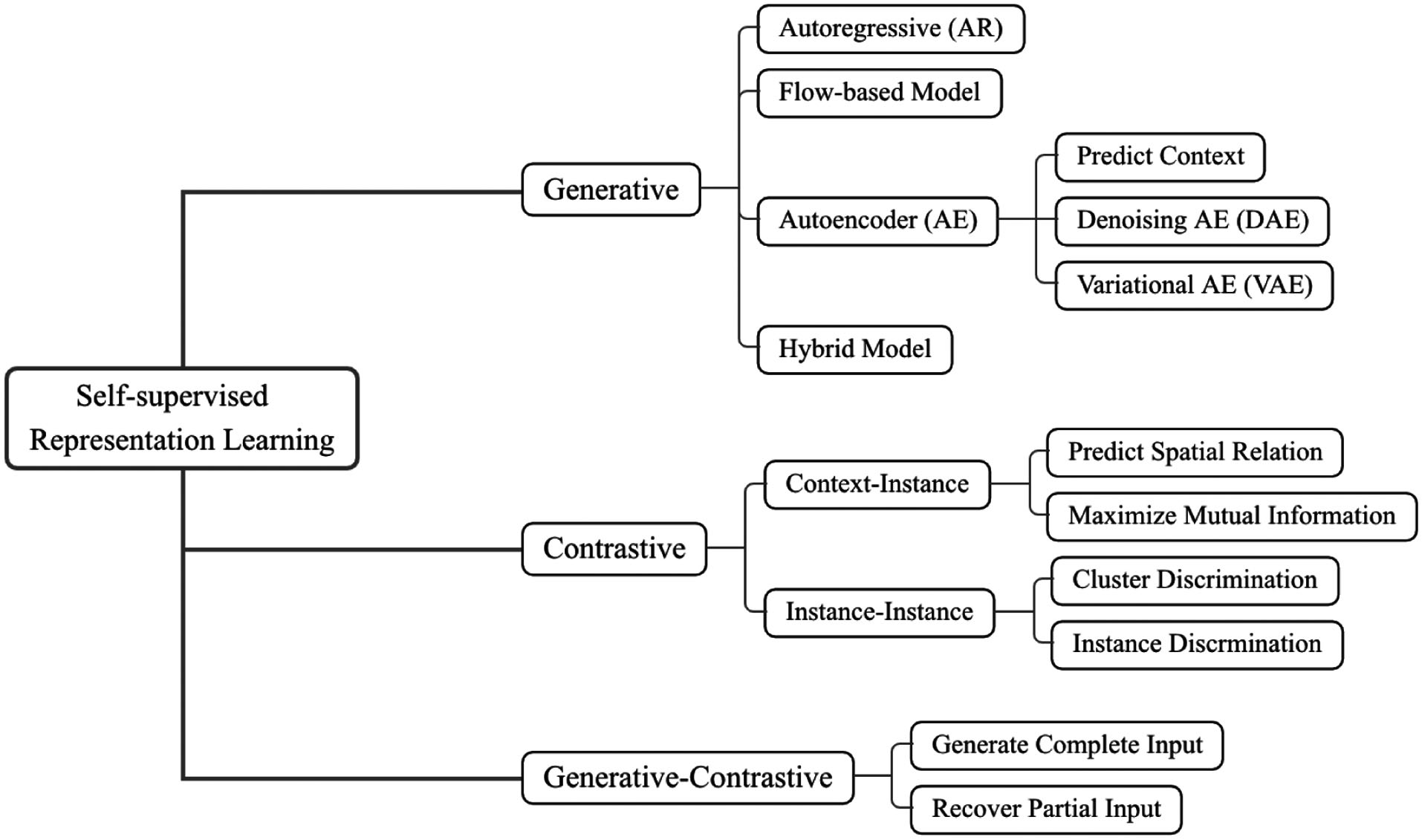 An extensive list of references on SSL can be found on GitHub. References
| ||||||||||||


Standardising/standardisation and whitening | ||||||||
|---|---|---|---|---|---|---|---|---|
Given a dataset , where denotes the number of samples and denotes the number of features, it is a common practice to preprocess so that each column has zero mean and unit variance; this is called standardising the data [Mur22, Sec. 7.4.5]. Standardising forces the variance (per column) to be 1 but does not remove correlation between columns. Decorrelation necessitates whitening. Whitening is a linear transformation of measurement that produces decorrelated such that the covariance matrix , where is called a whitening matrix [CPSK07, Sec. 2.5.3]. All , and have the same number of rows, denoted , which satisfies ; if , then dimensionality reduction is also achieved besides whitening. A whitening matrix can be obtained using eigenvalue decomposition:
where is an orthogonal matrix containing the covariance matrix’s eigenvectors as its columns, and is the diagonal matrix of the covariance matrix’s eigenvalues [ZX09, p. 74]. Based on the decomposition, the whitening matrix can be defined as
above is called the PCA whitening matrix [Mur22, Sec. 7.4.5]. References
| ||||||||


T |
|---|
Transfer learning | ||||||
|---|---|---|---|---|---|---|
References
| ||||||
Transformer | |||
|---|---|---|---|