Special | A | B | C | D | E | F | G | H | I | J | K | L | M | N | O | P | Q | R | S | T | U | V | W | X | Y | Z | ALL
A |
|---|
Activation function: contemporary options | ||||||||||||||||||||
|---|---|---|---|---|---|---|---|---|---|---|---|---|---|---|---|---|---|---|---|---|
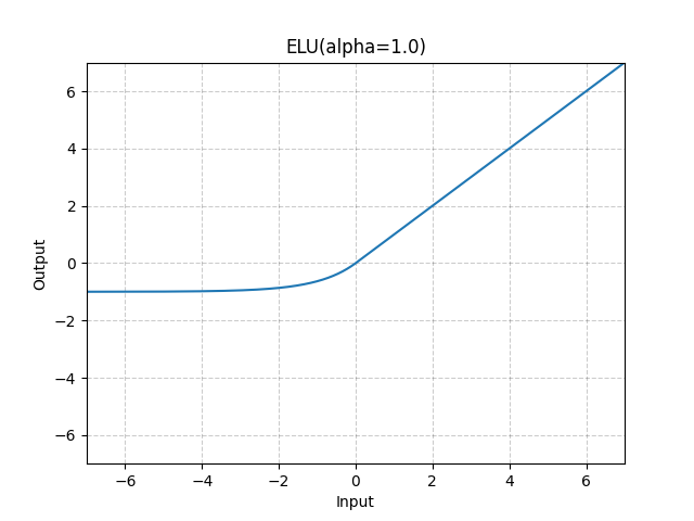
This knowledge base entry follows discussion of artificial neural networks and backpropagation. Contemporary options for are the non-saturating activation functions [Mur22, Sec. 13.4.3], although the term is not accurate. Below, should be understood as the output of the summing junction.
References
| ||||||||||||||||||||


 = \text{ReLU}(x) \triangleq \max(0,x) = \begin{cases}
x & \text{if }x>0, \\
0 & \text{otherwise.}
\end{cases}")

=0")

 = \text{LReLU}(x) \triangleq \max(ax,x) = \begin{cases}
x & \text{if }x>0, \\
ax & \text{otherwise,}
\end{cases}")


=a>0")
 = \text{PReLU}(x) \triangleq \max(ax,x) = \begin{cases}
x & \text{if }x>0, \\
ax & \text{otherwise,}
\end{cases}")
 = \text{ELU}(x) \triangleq \begin{cases}
x & \text{if }x>0, \\
\alpha(e^x-1) & \text{otherwise,}
\end{cases}")


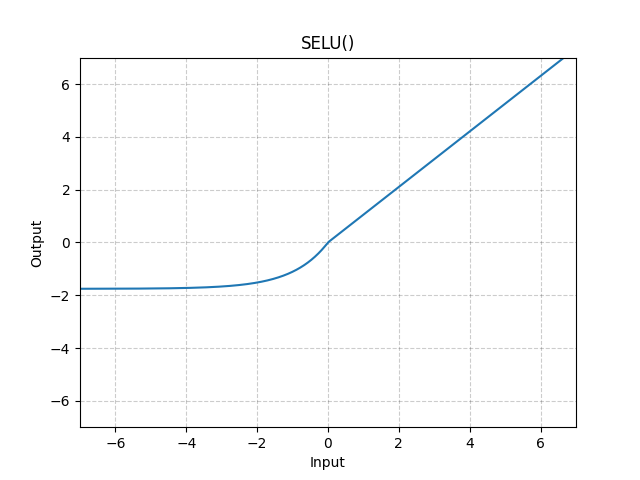
 = \text{SELU}(x) \triangleq \lambda\text{ELU}(x),")

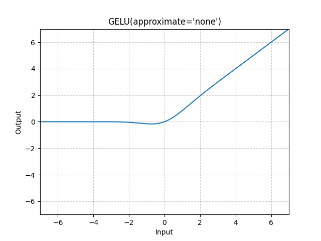
![\varphi(x) = \text{GELU}(x) \triangleq x\Phi(x) = \dfrac{x}{2}\left[1+\text{erf}(x/\sqrt{2})\right],](https://lo.unisa.edu.au/filter/tex/pix.php/2b58eace246ae23c0e4a88f1f8c72a50.gif "\varphi(x) = \text{GELU}(x) \triangleq x\Phi(x) = \dfrac{x}{2}\left[1+\text{erf}(x/\sqrt{2})\right],")
")

=(2/\sqrt{\pi})\int_0^xe^{-t^2}dt")
Active learning | ||
|---|---|---|
Adversarial machine learning | ||||||||
|---|---|---|---|---|---|---|---|---|
Adversarial machine learning (AML) as a field can be traced back to [HJN+11]. AML is the study of 1️⃣ the capabilities of attackers and their goals, as well as the design of attack methods that exploit the vulnerabilities of ML during the ML life cycle; 2️⃣ the design of ML algorithms that can withstand these security and privacy challenges [OV24]. The impact of adversarial examples on deep learning is well known within the computer vision community, and documented in a body of literature that has been growing exponentially since Szegedy et al.’s discovery [SZS+14]. The field is moving so fast that the taxonomy, terminology and threat models are still being standardised. See MITRE ATLAS. References
| ||||||||
Apache MXNet | ||
|---|---|---|
Deep learning library Apache MXNet reached version 1.9.1 when it was retired in 2023. Despite its obsolescence, there are MXNet-based projects that have not yet been ported to other libraries. In the process of porting these projects, it is useful to be able to evaluate their performance in MXNet, and hence it is useful to be able to set up MXNet. The problem is the dependencies of MXNet have not been updated for a while, and installation is not as straightforward as the installation guide makes it out to be. The installation guide here is applicable to Ubuntu 24.04 LTS on WSL2 and requires
After setting up all the above, do pip install mxnet-cu112
Some warnings like this will appear but are inconsequential: cuDNN lib mismatch: linked-against version 8907 != compiled-against version 8101. Set MXNET_CUDNN_LIB_CHECKING=0 to quiet this warning. | ||
Artificial neural networks and backpropagation | |||
|---|---|---|---|
See 👇 attachment.
| |||
Autoencoders | ||||||
|---|---|---|---|---|---|---|
An autoencoder References
| ||||||
B |
|---|
Batch normalisation (BatchNorm) | ||||||||||
|---|---|---|---|---|---|---|---|---|---|---|
Watch a high-level explanation of BatchNorm: Watch more detailed explanation of BatchNorm by Prof Ng: Watch coverage of BatchNorm in Stanford 2016 course CS231n Lecture 5 Part 2: References
| ||||||||||
C |
|---|
Convolutional neural networks | ||||||||||||||||||||||||||||||||
|---|---|---|---|---|---|---|---|---|---|---|---|---|---|---|---|---|---|---|---|---|---|---|---|---|---|---|---|---|---|---|---|---|
The convolutional neural network (ConvNet or CNN) is an evolution of the multilayer perceptron that replaces matrix multiplication with convolution in at least one layer[GBC16, Ch. 9]. A deep CNN is a CNN that has more than three hidden layers. CNNs play an important role in the history of deep learning because[GBC16, §9.11]:
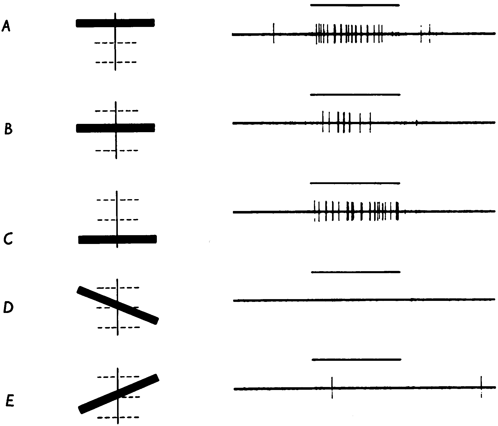
The following discusses the basic CNN structure and zooms in on the structural elements. StructureThe core CNN structure is inspired by the visual cortex of cats. The receptive field of a cell in the visual system may be defined as the region of retina (or visual field) over which one can influence the firing of that cell[HW62]. In a cat’s visual cortex, the majority of receptive fields can be classified as either simple or complex[HW62, LB02, Lin21]:
 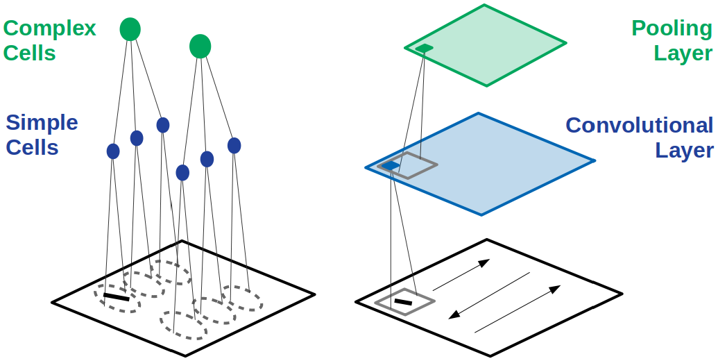 As a predecessor to the CNN, Fukushima’s neural network model “neocognitron”[Fuk80], as shown in Fig. 2, is a hierarchy of alternating layers of “S-cells” (modelling simple cells) and “C-cells” (modelling complex cells). The neocognitron performs layer-wise unsupervised learning (clustering to be specific)[GBC16, §9.10], such that none of the C-cells in the last layer responds to more than one stimulus pattern[Fuk80]. Furthermore, the response is invariant to the pattern’s position, small changes in shape or size[Fuk80]. Inspired by the neocognitron, the core CNN structure, as shown in Fig. 2, has convolution layers that mimic the behavior of S-cells, and pooling layers that mimic the behavior of C-cells. The output of a convolution layer is called a feature map[ZLLS23, §7.2.6]. Not shown in Fig. 2. is a nonlinear activation (e.g., ReLU) layer between the convolution layer and pooling layer; these three layers implement the three-stage processing that characterizes the CNN[GBC16, §9.3]. The nonlinear activation stage is sometimes called the detector stage[GBC16, §9.3]. Invariance to local translation is useful if detecting the presence of a feature is more important than localizing the feature. When it was introduced, the CNN brought three architectural innovations to achieve shift/translation-invariance[LB02, GBC16]:
 Structural element: convolutionIt has to be emphasised that the convolution in this context is inspired by but not equivalent to the convolution in linear system theory and furthermore it exists in several variants[GBC16, Ch. 9], but it is still a linear operation. In signal processing, if denotes a time-dependent input and denotes the impulse response function of a linear system, then the output response of the system is given by the convolution (denoted by symbol ) of and :
In discrete time, the equation above can be written as
Above, square brackets are used to distinguish discrete time from continuous time. In machine learning (ML), is called a kernel or filter and the output of convolution is an example of a feature map. For two-dimensional (2D) inputs (e.g., images), we use 2D kernels in convolution:
Convolution works similarly to windowed (Gabor) Fourier transforms[BK19, §6.5] and wavelet transforms[Mal16]. Convolution is not to be confused with cross-correlation, but for efficiency, convolution is often implemented as cross-correlation in ML libraries. For example, PyTorch implements 2D convolution (
Note above, the indices of are and instead of and . The absence of flipping of the indices makes cross-correlation more efficient. Both convolution and cross-correlation are invariant and equivariant to shift/translation. Both convolution and cross-correlation is neither scale- nor rotation-invariant[GBC16]. Instead of convolution, CNNs typically use cross-correlation because ... Fig. 4 animates an example of a cross-correlation operation using an edge detector filter. To an image, applying an filter at a stride of produces a feature map of size
assuming is a multiple of [Mad21].  Structural element: poolingA pooling function replaces the output of a neural network at a certain location with a summary statistic (e.g., maximum, average) of the nearby outputs[GBC16, §9.3]. The number of these nearby outputs is the pool width. Like a convolution/cross-correlation filter, a pooling window is slid over the input one stride at a time. Fig. 5 illustrates the maximum-pooling (max-pooling for short) operation[RP99]. Pooling helps make a feature map approximately invariant to small translations of the input. Furthermore, for many tasks, pooling is essential for handling inputs of varying size. Fig. 6 illustrates the role of max-pooling in downsampling. As a summary, Fig. 7 shows the structure of an example of an early CNN[LB02]. Note though the last layers of a modern CNN are typically fully connected layers (also known as dense layers).   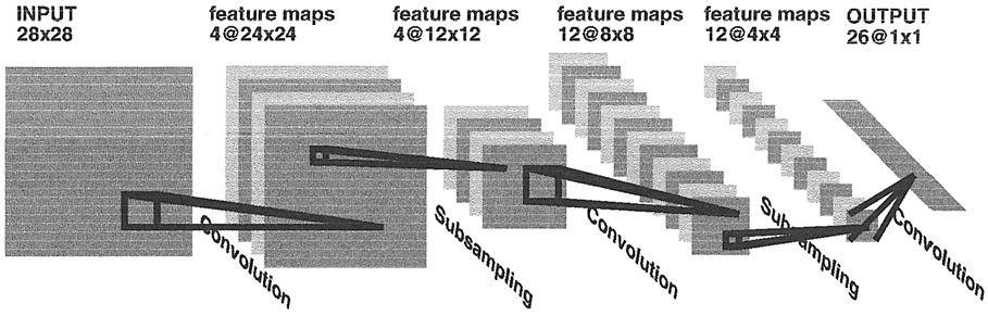 References
| ||||||||||||||||||||||||||||||||


")
")

(t) = \int_{\tau=0}^t x(\tau)f(t-\tau)d\tau.")
![(x\ast f)[t] = \sum_{\tau=0}^t x[t]\cdot f[t-\tau].](https://lo.unisa.edu.au/filter/tex/pix.php/c01e051d4cf9c3c14a9ac4572c941ede.gif "(x\ast f)[t] = \sum_{\tau=0}^t x[t]\cdot f[t-\tau].")
![(x\ast f)[i,j] = \sum_{a,b}x[a,b]\cdot f[i-a, j-b].](https://lo.unisa.edu.au/filter/tex/pix.php/c4936e08bd7cd6e79e2a4b337c9a3cf4.gif "(x\ast f)[i,j] = \sum_{a,b}x[a,b]\cdot f[i-a, j-b].")

![(x\star f)[i,j] = \sum_{a,b}x[i+a,j+b]\cdot f[a,b].](https://lo.unisa.edu.au/filter/tex/pix.php/821970207b3331adb054e91c5e092fd3.gif "(x\star f)[i,j] = \sum_{a,b}x[i+a,j+b]\cdot f[a,b].")


\times\left(\frac{n-m}{k}+1\right),")

Cross-entropy loss | ||||
|---|---|---|---|---|
[Cha19, pp. 11-14] References
| ||||
D |
|---|
Domain adaptation | |||
|---|---|---|---|
Domain adaptation is learning a discriminative classifier or other predictor in the presence of a shift of data distribution between the source/training domain and the target/test domain [GUA+16]. References | |||