Browse the glossary using this index

Special | A | B | C | D | E | F | G | H | I | J | K | L | M | N | O | P | Q | R | S | T | U | V | W | X | Y | Z | ALL

Page:  1  2  3  4  5  (Next)
  ALL

A

Picture of Yee Wei Law

Abstract algebra

by Yee Wei Law - Monday, 11 September 2023, 3:23 PM
 

See 👇 attachment or the latest source on Overleaf, on the topics of groups and Galois fields (pending).

Tags:

Picture of Yee Wei Law

Ancilla

by Yee Wei Law - Wednesday, 7 June 2023, 1:01 PM
 

An ancilla (system) is an auxiliary quantum-mechanical system [ETS18].

Think of ancilla as something extra that is used to achieve some goal [Pre18].

References

[ETS18] ETSI, Quantum Key Distribution (QKD); Vocabulary, Group Report ETSI GR QKD 007 v1.1.1, December 2018. Available at https://www.etsi.org/deliver/etsi_gr/QKD/001_099/007/01.01.01_60/gr_qkd007v010101p.pdf.
[Pre18] J. Preskill, Lecture Notes for Ph219/CS219: Quantum Information Chapter 3, 2018. Available at http://theory.caltech.edu/~preskill/ph219/chap2_15.pdf.
Tags:

Picture of Yee Wei Law

Axiomatic approach to quantum operations

by Yee Wei Law - Wednesday, 7 June 2023, 1:02 PM
 

In quantum information theory, the foundation of quantum cryptography, the concepts of general/generalised measurements and quantum channels are rooted in the concept of quantum operation [Pre18, Sec. 3.2.4].

  • A general measurement can be realised by entangling a system with a meter and performing a projective measurement on the meter.
  • A quantum channel arises if we measure the meter but completely forget the measurement outcome.

While the time evolution of a closed quantum system can be expressed using a single unitary operator, the time evolution of an open quantum system is much less straightforward [HXK20], and this is where the theory of quantum operations come in.

Here, the axiomatic approach in [NC10, Sec. 8.2.4] to defining quantum operations is discussed, starting with Definition 1.

Definition 1: Quantum operation [NC10, p. 367]

A quantum operation is a map from the set of density operators for the input space to the set of density operators for the output space , that satisfies these axioms:

Axiom 1

, with value between 0 and 1 inclusive, is the probability that the process represented by occurs, when is the initial state.

💡 Recall Eq. (1) in the discussion of density operator.

Axiom 2

is a convex-linear map on the set of density operators, i.e., for probabilities ,

Axiom 3

is a completely positive map, i.e., if maps density operators of system to density operators of system , then must be positive for any positive operator .

Furthermore, if we introduce an extra system of arbitrary dimensionality, then , where denotes the identity map on system , is positive for any positive operator on the combined system .

Justification of Axiom 1: In the absence of measurement, by itself completely describes the quantum operation, and Axiom 1 reduces to the requirement that ; in this case, the quantum operation is trace-preserving.

  • If does not completely describe the operation, then there exists such that , and is so-called non-trace-preserving.
  • Every physical quantum operation on satisfies the requirement that .

Justification of Axiom 2: Let , then

where is a normalisation factor.

By Bayes’ rule,

Justification of Axiom 3: A quantum operation maps a density operator to a density operator — by itself or as part of a larger system — and density operators are always positive, so must be a completely positive map.

Example 1 [Pre18, p. 19]

This example is meant to show that the transpose operation is not a completely positive map and hence not a quantum operation.

We first observe that is positive if is positive because the quadratic form

However, the transpose operation is not completely positive due to the following.

Suppose system contains entangled subsystems and , and has state , ignoring the normalisation constant.

The density matrix of is

Above, we applied the identity .

Now consider the composite map , where is the transpose operation, which transforms to .

Applying the composite map to , we get

Applying the composite map to the above, we get back

Therefore, if we represent the map with a square matrix, the matrix is involutory (square = identity), and it is trivial to show that the eigenvalues of an involutory matrix are (see below), implying the composite map is not positive.

Note: For involutory , .

In other words, the transpose operation is not a completely positive map, and hence not a quantum operation.

Axioms 1-3 lead to the following important theorem.

Theorem 1 [NC10, Theorem 8.1]

The map satisfies Axioms 1-3 if and only if

(1)

for some set of operators that map the input Hilbert space to the output Hilbert space, and .

In Theorem 1,

  • The statement is equivalent to the statement is positive-semidefinite.
  • are so-called Kraus operators or operation elements [Pre18, Sec. 3.2.1], and Eq. (1) is called an operator-sum representation of [MM12, Sec. 2.14].
    • Operator-sum representations are not unique because of the unitary freedom in these representations [NC10, Theorem 8.2]; see Example 2.
  • If , then form a POVM [WN17, Definition 1.5.2], and we have a nonunique Kraus decomposition of .
    • A Kraus decomposition always exists for POVM by simply setting , the positive square root of (Python function scipy.lingalg.sqrtm, MATLAB function sqrtm).
    • If is a projector, then and we can set .
Example 2 [MM12, p. 176]

Consider the Kraus operators or operation elements: and , where .

An equivalent operator-sum representation can be provided by and , because

The freedom in the operator-sum representation is especially useful for studying quantum error correction.

Theorem 2 [NC10, Theorem 8.3]

Any quantum operation on a system of -dimensional Hilbert space can be generated by an operator-sum representation containing at most elements:

where .

Watch lectures on Kraus representations by Artur Ekert, inventor of the E91 QKD protocol:

References

[HXK20] Z. Hu, R. Xia, and S. Kais, A quantum algorithm for evolving open quantum dynamics on quantum computing devices, Sci Rep 10 (2020), 3301. https://doi.org/10.1038/s41598-020-60321-x.
[MM12] D. C. Marinescu and G. M. Marinescu, Classical and Quantum Information, Elsevier, 2012. https://doi.org/10.1016/C2009-0-64195-7.
[NC10] M. A. Nielsen and I. L. Chuang, Quantum computation and quantum information, 10th anniversary ed., Cambridge University Press, 2010. Available at http://mmrc.amss.cas.cn/tlb/201702/W020170224608149940643.pdf.
[Pre18] J. Preskill, Lecture Notes for Ph219/CS219: Quantum Information Chapter 3, 2018. Available at http://theory.caltech.edu/~preskill/ph219/chap2_15.pdf.
[WN17] S. Wehner and N. Ng, Lecture Notes: edX Quantum Cryptography, CaltechDelftX: QuCryptox, 2017. Available at https://courses.edx.org/courses/course-v1:CaltechDelftX+QuCryptox+3T2018/pdfbook/0/.
Tags:

B

Picture of Yee Wei Law

BB84: Overview

by Yee Wei Law - Thursday, 26 October 2023, 2:27 PM
 

Quantum key distribution (QKD) is a method for generating and distributing symmetric cryptographic keys with information-theoretic security based on quantum information theory [ETS18].

A QKD protocol establishes a secret key between two parties — let us call them 👩 Alice and 🧔 Bob as per tradition — connected by 1️⃣ an insecure quantum channel and 2️⃣ an authenticated classical channel [Gra21, Sec. 3.1].

  • The established key can be however long as required so that it can serve as the key in a one-time pad.
  • “Authenticated” does not imply “confidential” and does not necessarily require the use of cryptography. Alice and Bob can physically meet and verify each other’s identity.
  • In practice, the authenticated classical channel can be established using 1️⃣ a pre-shared symmetric key, or 2️⃣ public-key cryptography [PAB+20, Sec. F].

A QKD protocol typically proceeds in two phases [Wol21, Ch. 4]:

  1. the quantum transmission phase, in which 👩 Alice and 🧔 Bob send and/or measure quantum states;
  2. the classical post-processing phase, where the bitstrings generated in the previous phase are converted into a pair of secret keys.

The security of QKD hinges on the principles of quantum mechanics, rather than the hardness of any computational problem, and hence does not get threatened by advances in computing technologies.

  • During the quantum transmission phase, any adversary — let us call it 😈 Eve as per tradition — eavesdropping on the quantum channel inherently disturbs the channel and interrupts the key establishment process.
  • Eve cannot make a copy of any transmitted state (that contributes to the key to be established) thanks to the no-cloning theorem.
Theorem 1: No-cloning theorem [WZ82]

It is not possible to perfectly clone an unknown quantum state.

The earliest QKD protocol is due to Bennett and Brassad [BB84] and is called BB84, named after the authors and the year it was proposed.

QKD leverages physical mechanisms, so unavoidably we need to discuss the physical mechanisms that underlie/enable BB84, which are based primarily on the polarisation of photons [Wol21, Sec. 1.3.1].

Polarisation

The polarisation of photons specifies the geometrical orientation of the oscillation of its electromagnetic field.

  • Polarisation is linear if the field only oscillates in one direction.
  • Polarisation is circular if the field rotates in a plane as the wave propagates.

We only consider linear polarisation here. For linear polarisation, we distinguish between two bases:

  • rectilinear basis, which includes horizontal and vertical orientations; and
  • diagonal basis, which is essentially the rectilinear basis rotated by ; as shown in Fig. 1.
Fig. 1: Polarisation bases and filters [Wol21, Fig. 1.4].

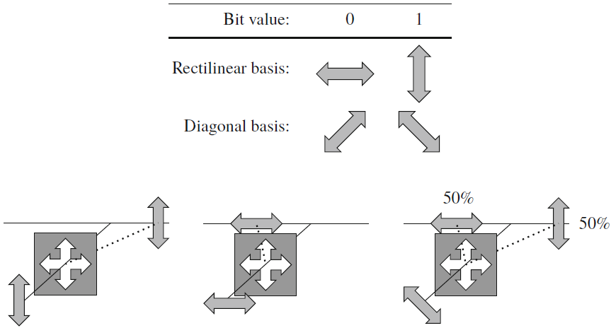
Consider the effect of polarisation filters depicted in Fig. 1:

  • When a ↕ vertically polarised photon passes through a rectilinear polarisation filter, it is deflected to the right (➡).
  • When a ↔ horizontally polarised photon passes through a rectilinear polarisation filter, it is deflected to the left (⬅).
  • When a diagonally polarised photon passes through a rectilinear polarisation filter, it is equally likely to be deflected to the left and right.

Thus, measuring a diagonally polarised photon in the rectilinear basis, and similarly measuring a vertically/horizontally polarised photon in the diagonal basis, give a random result.

  • We call the rectilinear and diagonal bases mutually conjugate (see Definition 1).

    Definition 1: Conjugate bases

    Two bases are mutually conjugate [BB84; FGG+97] or unbiased [Wol21, p. 9] if each vector of one basis has equal-length projections onto all vectors of the other basis.

  • The Heisenberg uncertainty principle ensures that when making two sequential measurements using conjugate bases, the system is disturbed in such a way that the uncertainty of the measurement outcome is maximised [Woj22, p. 42].

With knowledge of polarisation in mind, let us now discuss the quantum transmission phase of BB84, which involves encoding of classical bits into quantum states, communication over a quantum channel, and decoding of quantum states into classical bits.

Quantum transmission phase

This phase of the protocol involving 👩 Alice and 🧔 Bob goes like this [Wol21, Sec. 1.3.2]:

  1. 👩 Alice chooses a string of random classical bits: .
  2. 👩 Alice chooses a random sequence of rectilinear (Z) bases and diagonal (X) bases; these are called the canonical bases [Dua14, p. 295].
  3. 👩 Alice encodes her bitstring into a collection of photons with basis-dependent polarisation.

    In the rectilinear basis, 0 and 1 are encoded as → and ↑ respectively.

    In the diagonal basis, 0 and 1 are encoded as ↗ and ↖ respectively.

  4. When 🧔 Bob receives the photons, he randomly (and independently of Alice) decides for each photon whether to measure/decode it in the rectilinear or diagonal basis to retrieve the classical bit.
  5. At the end of this quantum transmission phase, 👩 Alice and 🧔 Bob each holds a classical bit string, denoted for Alice and for Bob. and form the raw key pair.

An illustration of the process above can be found Fig. 1.

Fig. 1: In steps 1-3, 👩 Alice and 🧔 Bob engage in the quantum transmission phase, while 😈 Eve eavesdrops on the transmission and attempts to recover the raw key bits. ⚠ The mapping of 0 and 1 in the diagonal basis illustrated here is different from that in the earlier discussion, which follows the original paper [BB84]. In steps 4-5, 👩 Alice and 🧔 Bob engage in the sifting step, discussed in the next section. Diagram from [LCPP22, Fig. 2a].

Since the polarisation state of each photon is a discrete variable, BB84 is an example of a discrete-variable quantum key distribution (DV-QKD) scheme.

BB84 is also an example of a prepare-and-measure protocol, because of the preparation action of 👩 Alice and the measurement action of 🧔 Bob.

Classical post-processing phase

This phase of the protocol involves 👩 Alice and 🧔 Bob exchanging a sequence of classical information in the classical channel to transform their raw key pair into a shared secret key [Wol21, Sec. 1.3.3]:

  1. This is the sifting step (steps 4-5 in Fig. 1):
    • 🧔 Bob publicly announces the bases he has chosen to measure the photons Alice has sent.
    • 👩 Alice compares Bob’s bases to the ones she used and confirms which bases Bob has chosen correctly.
    • 👩 Alice and 🧔 Bob discard all the bits for which the encoding and measurement bases are not the same.
  2. This is the parameter estimation step:
    • 👩 Alice and 🧔 Bob want to compute an estimate of the quantum bit error rate (QBER) in the quantum channel, i.e., the fraction of bits where and differ in the Z and X bases [Gra21, p. 38].
    • For this, 🧔 Bob reveals a random subset of his key bits.
    • In case of no eavesdropping, these bits should be the same as Alice’s bits and 👩 she confirms them.
    • If the QBER is too high, 👩 Alice and 🧔 Bob suspect eavesdropping and abort the protocol.
    • The bits that have been revealed during this step are discarded as their information is now public to eavesdroppers.
  3. Computation of the final key if the error rate is not too high:
    • 👩 Alice and 🧔 Bob perform steps, which were later additions to the original BB84 [BBR88], to correct errors in their keys and increase the secrecy of their key.
    • The first step is error correction (also called information reconciliation), where they erase all errors in their bit strings. After this step, they hold identical strings.

      Direct vs reverse reconciliation [GG02; Djo19, p. 7; PAB+20, Sec. B]

      ▶ Direct reconciliation: 👩 Alice sends correction information and 🧔 Bob corrects his key elements to have the same values as Alice’s.

      • For example, 👩 Alice performs low-density parity check (LDPC) encoding and sends the parity bits to 🧔 Bob, who in turn performs LDPC decoding.
      • Error correction fails when quantum channel loss exceeds 50%.

      ◀ Reverse reconciliation: 🧔 Bob sends correction information and 👩 Alice corrects her key elements to have the same values as Bob’s.

      • For example, 🧔 Bob performs LDPC encoding and sends the parity bits to 👩 Alice, who in turn performs LDPC decoding.
      • Preferred option to direct reconciliation.
      • Provides a usable key when the mutual information of Alice () and Bob () exceeds the mutual information of Bob and Eve (), i.e., ; the difference between these two terms gives the asymptotic secret key rate.
    • The second step is privacy amplification, which is a procedure that minimises Eve’s knowledge of the key.

Table 1 shows an example of an exchange between 👩 Alice and 🧔 Bob in the absence of eavesdropping.

Table 1: An example of an exchange between 👩 Alice and 🧔 Bob in BB84 in the absence of eavesdropping [Wol21, Table 1.2].

For discussion of physical realisations of BB84, follow this knowledge base entry.

Performance and security evaluation

In terms of performance, a basic figure of merit of every QKD protocol is the secret key rate, i.e. the fraction of secure key bits produced per protocol round.

For security, follow this overview of QKD security.

References

[BB84] C. H. Bennett and G. Brassard, Quantum cryptography: Public key distribution and coin tossing, in Proceedings of the International Conference on Computers, Systems & Signal Processing, December 1984, pp. 175–179. Available at https://arxiv.org/abs/2003.06557.
[BBR88] C. H. Bennett, G. Brassard, and J.-M. Robert, Privacy amplification by public discussion, SIAM Journal on Computing 17 no. 2 (1988), 210–229. Available at https://www.proquest.com/docview/919828123.
[Djo19] I. B. Djordjevic, Physical-Layer Security and Quantum Key Distribution, Springer Cham, 2019. https://doi.org/10.1007/978-3-030-27565-5.
[Dua14] F. Duarte, Quantum Optics for Engineers, CRC Press, 2014. https://doi.org/10.1201/b16055.
[ETS18] ETSI, Quantum Key Distribution (QKD); Vocabulary, Group Report ETSI GR QKD 007 v1.1.1, December 2018. Available at https://www.etsi.org/deliver/etsi_gr/QKD/001_099/007/01.01.01_60/gr_qkd007v010101p.pdf.
[FGG+97] C. A. Fuchs, N. Gisin, R. B. Griffiths, C.-S. Niu, and A. Peres, Optimal eavesdropping in quantum cryptography. i. information bound and optimal strategy, Phys. Rev. A 56 no. 2 (1997), 1163–1172. https://doi.org/10.1103/PhysRevA.56.1163.
[Gra21] F. Grasselli, Quantum Cryptography: From Key Distribution to Conference Key Agreement, Quantum Science and Technology, Springer Cham, 2021. https://doi.org/10.1007/978-3-030-64360-7.
[GG02] F. Grosshans and P. Grangier, Reverse reconciliation protocols for quantum cryptography with continuous variables, arXiv preprint quant-ph/0204127, 2002. https://doi.org/10.48550/arXiv.quant-ph/0204127.
[LCPP22] C.-Y. Lu, Y. Cao, C.-Z. Peng, and J.-W. Pan, Micius quantum experiments in space, Rev. Mod. Phys. 94 no. 3 (2022), 035001. https://doi.org/10.1103/RevModPhys.94.035001.
[PAB+20] S. Pirandola, U. L. Andersen, L. Banchi, M. Berta, D. Bunandar, R. Colbeck, D. Englund, T. Gehring, C. Lupo, C. Ottaviani, J. L. Pereira, M. Razavi, J. Shamsul Shaari, M. Tomamichel, V. C. Usenko, G. Vallone, P. Villoresi, and P. Wallden, Advances in quantum cryptography, Advances in Optics and Photonics 12 no. 4 (2020), 1012–1236. https://doi.org/10.1364/AOP.361502.
[Woj22] F. Wojcieszyn, Introduction to Quantum Computing with Q# and QDK, Quantum Science and Technology, Springer Cham, 2022. https://doi.org/10.1007/978-3-030-99379-5.
[Wol21] R. Wolf, Quantum Key Distribution: An Introduction with Exercises, Springer, Cham, 2021. https://doi.org/10.1007/978-3-030-73991-1.
[WZ82] W. K. Wootters and W. H. Zurek, A single quantum cannot be cloned, Nature 299 no. 5886 (1982), 802–803. https://doi.org/10.1038/299802a0.
Tags:

Picture of Yee Wei Law

BB84: Physical realisations

by Yee Wei Law - Thursday, 26 October 2023, 5:47 PM
 
Acknowledgement: Andrew Edwards contributed some explanation.

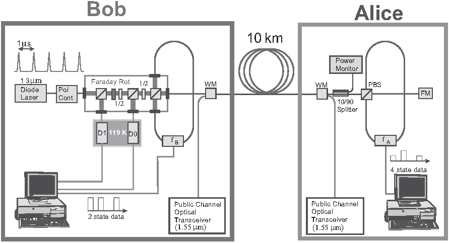
Continuing from an overview of BB84, this entry discusses several ways in which BB84 can be realised.

Fig. 1 shows an experimental setup built by IBM [NC10, Box 12.7], where

  • 🧔 Bob generates strong coherent states using a 1.3 μm (near infrared wavelength) diode laser and transmits the states to 👩 Alice 10 km away via an optical fibre.
  • 👩 Alice attenuates the states to generate approximately a single photon, and subsequently polarises the photon to one of , , and .
  • 👩 Alice returns the photon to 🧔 Bob, who measures it using a polarisation analyser in a random basis (either rectilinear or diagonal).
Fig. 1: An experimental setup for BB84 built by IBM [NC10, Box 12.7]. The setup achieved a key bit rate of several hundred bits per second, which is far from practical but it was a start.

For the setup in Fig. 1,

  • The reason for making the photons traverse the optical fibre twice (from Bob to Alice then back to Bob) is to automatically compensate for asymmetry and fluctuations of the medium.
  • The polarisation controller (“Pol Cont” in Fig. 1) is for correcting polarisation drifts in the quantum channel [Sud10, p. 111].
  • The Faraday rotator (“Faraday Rot” in Fig. 1) effects polarisation through the Faraday (rotation) effect; watch demonstration on YouTube.
  • The classical channel of wavelength 1.55 μm is carried over the same optical fibre. Multiplexing of the quantum and classical channels is achieved through the wavelength (division) multiplexers (“WM” in Fig. 1).
  • The polarising beamsplitter (also called polarization beamsplitter, or “PBS” in Fig. 1) plays a crucial role, but let us first look at Thorlabs’ Quantum Cryptography Analogy Demonstration Kit (part number EDU-QCRY1), because the accompanying manual [Tho20] is rich with practical information rarely found elsewhere.

Fig. 2 shows a minimalist block diagram for EDU-QCRY1, while Fig. 3 shows a photo of a physical setup realising the block diagram.

Fig. 2: A minimalist block diagram for Thorlab’s EDU-QCRY1.
Fig. 3: A photo of a physical setup implementing the block diagram in Fig. 2. The silver boxes with a red button are laser electronics. The silver boxes with a green button are sensor electronics. The silver boxes with no button are photon detectors. In EDU-QCRY1, pulsed light sources are used to approximate single-photon sources; see the risk of this approximation in terms of the photon number splitting attack.

Let us study the functions of the PBS in this context:

  • For Alice to send a to Bob, a half-wave plate (HWP, also called λ/2 plate, labelled as “Polarization Rotator” in Fig. 4) is physically rotated to 0°.

    Fig. 4: Transmission from Alice to Bob in the rectilinear basis [Tho20, Figure 2].

    To send a , the HWP is physically rotated by 45° to achieve a polarisation rotation of 90°.

    In general, for linearly polarised light, polarisation is rotated by a value twice as large as the rotation of the HWP.

  • On Bob’s side, a horizontally polarised photon () passes through the PBS, while a vertically polarised photon () gets reflected, as shown:

    Fig. 5: The effect of a PBS cube [Tho20, p. 21].

    Thus, a single-photon detector is needed to detect each state.

  • To support both the rectilinear basis (0° and 90°) and diagonal basis (-45° and 45°), the setup in Fig. 4 is extended to the setup in Fig. 6, where Alice’s polarisation rotator now support four angles in total (, , , ), and Bob gets a polarisation rotator that supports two angles (one for each basis).

    Fig. 6: Transmission from Alice to Bob in two bases (0° and 90°, -45° and 45°) [Tho20, Figure 3].

    Note Bob still needs only two photon detectors, one for each basis state of the selected basis.

  • Eve can be emulated by simply 1️⃣ duplicating the setup for Bob (for intercepting Alice’s photons), and 2️⃣ duplicating the setup for Alice (for “replaying” measured states to Bob); as shown in Fig. 2.

In recent years, satellite-based experiments on BB84 and extensions of BB84 (e.g., decoy-state BB84) had been conducted [LCPP22].

Compared to free space, polarisation is harder to preserve over commercial optical fibres [GK05, Fig. 11.7]. An alternative approach to polarisation is using an interferometer, such as a Mach-Zehnder interferometer; see Fig. 7 and [HIP+21, Sec. 3.2].
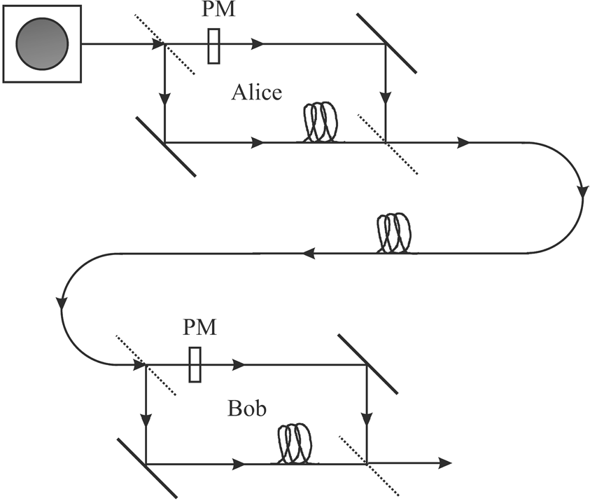
Fig. 7: Realising BB84 using an interferometer [GK05, Fig. 11.7]. The shorter and longer paths through the interferometer define the 0 and 1 states. Phase modulators (PM) are positioned within the upper arms of both Bob’s and Alice’s interferometer.

References

[GK05] C. Gerry and P. Knight, Introductory Quantum Optics, Cambridge University Press, 2005. https://doi.org/10.1017/CBO9780511791239.
[HIP+21] C. Hughes, J. Isaacson, A. Perry, R. F. Sun, and J. Turner, Quantum Computing for the Quantum Curious, Springer Cham, 2021. https://doi.org/10.1007/978-3-030-61601-4.
[LCPP22] C.-Y. Lu, Y. Cao, C.-Z. Peng, and J.-W. Pan, Micius quantum experiments in space, Rev. Mod. Phys. 94 no. 3 (2022), 035001. https://doi.org/10.1103/RevModPhys.94.035001.
[NC10] M. A. Nielsen and I. L. Chuang, Quantum computation and quantum information, 10th anniversary ed., Cambridge University Press, 2010. Available at http://mmrc.amss.cas.cn/tlb/201702/W020170224608149940643.pdf.
[Sud10] M. Suda, QKD Systems, in Applied Quantum Cryptography (C. Kollmitzer and M. Pivk, eds.), Lect. Notes Phys. 797, Springer Berlin Heidelberg, 2010, pp. 71–95. https://doi.org/10.1007/978-3-642-04831-96.
[Tho20] Thorlabs, EDU-QCRY1 EDU-QCRY1/M: Quantum Cryptography Demonstration Kit: Manual, December 2020. Available at https://www.thorlabs.com/_sd.cfm?fileName=MTN005660-D02.pdf&partNumber=EDU-QCRY1.
Tags:

Picture of Yee Wei Law

Bell states

by Yee Wei Law - Thursday, 8 June 2023, 11:31 PM
 

Consider the circuit below, where a Hadamard gate is connected to qubit and a controlled-NOT (CNOT) gate is connected to after the Hadamard gate:

Fig. 1: Quantum circuit for generating Bell states.

The Hadamard gate in Fig. 1 effects the transformations: and .

The CNOT gate in Fig. 1 has its control qubit connected to the line, and its target qubit connected to the line.

The unitary matrix representing the CNOT gate is

If the input to the CNOT gate is the state , then the output is

Thus, as an example, if the input is , then the Hadamard gate transforms it to , and the CNOT gate further transforms it to

Table 1 is the truth table summarising the outputs corresponding to basis-state inputs.

Table 1: Truth table for quantum circuit in Fig. 1.
Input Output

The output states in Table 1 are called the Bell states or Einstein-Podolsky-Rosen (EPR) pairs [KLM07, p. 75; NC10, Sec. 1.3.6], and can be represented concisely as

When the Bell states are used as an orthonormal basis, they are called the Bell basis [Wil17, pp. 91-93].

References

[KLM07] P. Kaye, R. Laflamme, and M. Mosca, An Introduction to Quantum Computing, Oxford University Press, 2007. Available at https://ebookcentral.proquest.com/lib/ unisa/reader.action?docID=415080.
[NC10] M. A. Nielsen and I. L. Chuang, Quantum computation and quantum information, 10th anniversary ed., Cambridge University Press, 2010. Available at http://mmrc.amss.cas.cn/tlb/201702/W020170224608149940643.pdf.
[Wil17] M. M. Wilde, Quantum Information Theory, 2nd ed., Cambridge University Press, 2017. https://doi.org/10.1017/9781316809976.
Tags:

Picture of Yee Wei Law

Bloch sphere

by Yee Wei Law - Thursday, 24 August 2023, 12:24 PM
 

Consider the ket vector , where and are complex-valued probability amplitudes, and are the computational bases.

We can express and in the exponential form [Wil17, (3.6)]:

we can rewrite as

where is related to and by:

Thus, given , we can rewrite it in the physically equivalent form:

where , , . Note:

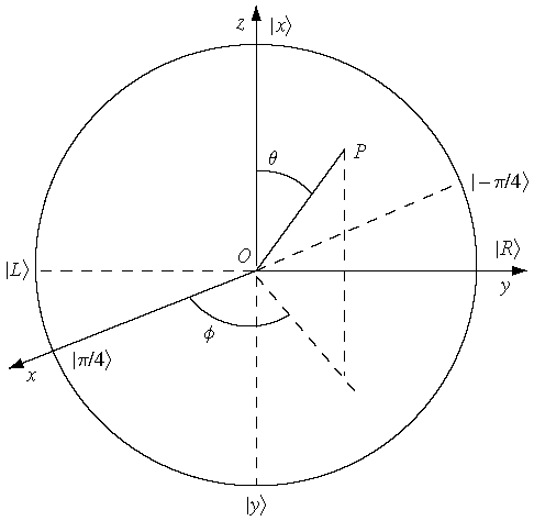
💡 Above, is used instead of because for visualisation using a Bloch sphere (more on this later), as ranges from 0 to , the values of and are confined within to ensure the qubit representation is unique [Wil17, p. 57].

So what is a Bloch sphere?

Named after physicist Felix Bloch, a Bloch sphere is a unit-radius sphere for visualising a qubit relative to the computational basis states.

Fig. 1: Ket-vector visualised in a Bloch sphere featuring computational basis states and [Wil17, Figure 3.2].

As shown in Fig. 1,

  • The north and south poles are typically chosen to represent and respectively, or the spin-up and spin-down states of an electron respectively.
  • Orthogonal states like and do not appear to be geometrically orthogonal in a Bloch sphere.
  • The angles and represent the polar and azimuthal angles respectively [Le 06, Sec. 3.1].
  • The , and coordinates of a ket vector on the Bloch sphere are not as meaningful.
  • Every point on the equator represents an equally weighted superposition of and .

As explained in Fig. 2, a sphere provides the necessary number of degrees of freedom to represent a ket vector.

Fig. 2: Why Bloch sphere?

The equator of a Bloch sphere enables the representation of complementary bases. For example, in Fig. 3,

  • (, undetermined) and (, undetermined) represent the basis states for linear polarisations along two perpendicular axes [Le 06, p. 12].
  • (, ) and (, ) represent the basis states for circular polarisation, [Le 06, p. 33].
  • and are complementary bases, which play a crucial role in quantum key distribution.
Fig. 3: A Bloch sphere featuring photon polarisation bases , and [Le 06, Figure 3.1]

References

[Le 06] M. Le Bellac, A Short Introduction to Quantum Information and Quantum Computation, Cambridge University Press, 2006. https://doi.org/10.1017/CBO9780511755361.
[Wil17] M. M. Wilde, Quantum information theory, 2nd ed., Cambridge University Press, 2017. https://doi.org/10.1017/9781316809976.
Tags:

C

Picture of Yee Wei Law

Coherent attack

by Yee Wei Law - Tuesday, 29 August 2023, 5:25 PM
 

The discussion here follows from the discussion of collective attacks.

Tags:

Picture of Yee Wei Law

Coherent state

by Yee Wei Law - Thursday, 26 October 2023, 4:16 PM
 

A coherent state is a special quantum state that a coherent laser ideally emits [Wil07, p. 19].

That 👆 does not say much, but there is no straightforward way to define “coherent state”, a concept introduced by Schrödinger [SZ97, p. 46].

Mathematically and in short, a coherent state is the eigenstate of the positive frequency part of the electric field operator [SZ97, p. 46], but this requires definition of the electric field operator, which in turn requires discussion of the quantization of electromagnetic fields.

Classically, an electromagnetic field consists of waves with well-defined amplitude and phase, but in quantum mechanics, this is no longer true.

More precisely, there are fluctuations in both the amplitude and phase of the field [SZ97, Ch. 2].

coherent state is a state that has the same fluctuations of quadrature amplitudes as the vacuum state but which possibly has nonzero average quadrature amplitudes [Van06, Sec. 4.6.1].

References

[GK05] C. Gerry and P. Knight, Introductory Quantum Optics, Cambridge University Press, 2005. https://doi.org/10.1017/CBO9780511791239.
[SZ97] M. O. Scully and M. S. Zubairy, Quantum Optics, Cambridge University Press, 1997. https://doi.org/10.1017/CBO9780511813993.
[Van06] G. Van Assche, Quantum Cryptography and Secret-Key Distillation, Cambridge University Press, 2006. https://doi.org/10.1017/CBO978051161.
[Wil07] M. M. Wilde, Quantum Information Theory, 2nd ed., Cambridge University Press, 2017. https://doi.org/10.1017/9781316809976.
Tags:

Picture of Yee Wei Law

Collective attack

by Yee Wei Law - Tuesday, 29 August 2023, 5:24 PM
 

The discussion here follows from the discussion of individual attacks.

In a collective attack [Sch10],

  • Eve prepares an ancilla state for each signal coming from Alice and lets it interact with the signal.

  • Eve passes Alice’s signal on to Bob.

References

[ETS18] ETSI, Quantum Key Distribution (QKD); Vocabulary, Group Report ETSI GR QKD 007 v1.1.1, December 2018. Available at https://www.etsi.org/deliver/etsi_gr/QKD/001_099/007/01.01.01_60/gr_qkd007v010101p.pdf.
[Sch10] S. Schauer, Attack Strategies on QKD Protocols, in Applied Quantum Cryptography (C. Kollmitzer and M. Pivk, eds.), Lect. Notes Phys. 797, Springer Berlin Heidelberg, 2010, pp. 71–95. https://doi.org/10.1007/978-3-642-04831-9_5.
[Wol21] R. Wolf, Quantum Key Distribution: An Introduction with Exercises, Springer, Cham, 2021. https://doi.org/10.1007/978-3-030-73991-1.
Tags:


Page:  1  2  3  4  5  (Next)
  ALL