Browse the glossary using this index

Special | A | B | C | D | E | F | G | H | I | J | K | L | M | N | O | P | Q | R | S | T | U | V | W | X | Y | Z | ALL

S

Picture of Yee Wei Law

Self-supervised learning

by Yee Wei Law - Tuesday, 25 April 2023, 10:20 AM
 

In his 2018 talk at EPFL and his AAAI 2020 keynote speech, Turing award winner Yann LeCun referred to self-supervised learning (SSL, not to be confused with Secure Socket Layer) as an algorithm that predicts any parts of its input for any observed part.

A standard definition of SSL remains as of writing elusive, but it is characterised by [LZH+23, p. 857]:

  • derivation of labels from data through a semi-automatic process;
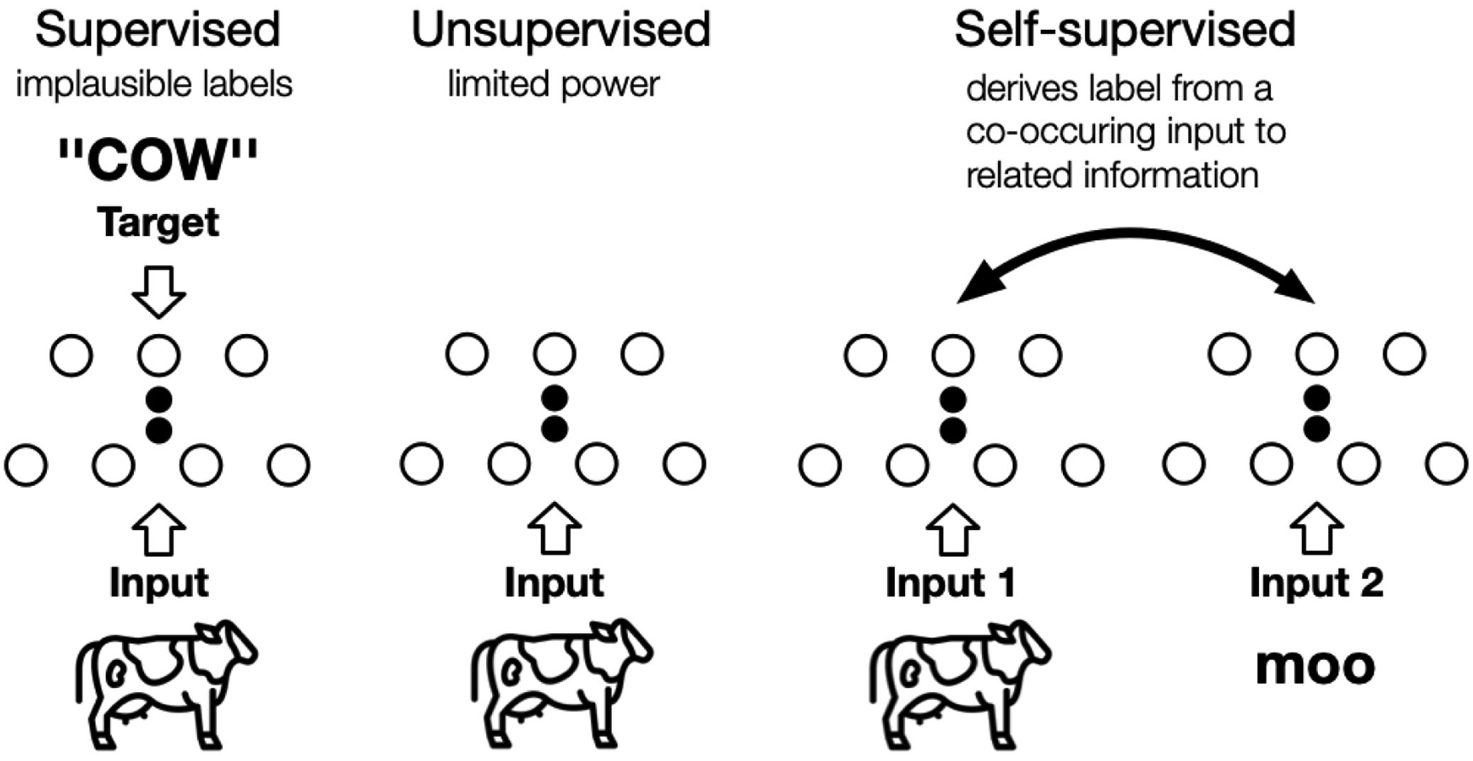
  • prediction of parts of the data from other parts, where “other parts” could be incomplete, transformed, distorted or corrupted (see Fig. 1).
Fig. 1: Unlike supervised and unsupervised learning, in self-supervised learning, the related, co-occurring information in “Input 2” is used to derive training labels [LZH+23, Fig. 1]. This related information can be a different modality of “Input 1”, or parts of “Input 1”, or another form of “Input 1”.

SSL can be understood as learning to recover parts or some features of the original input, hence it is also called self-supervised representation learning.

SSL has two distinct phases (see Fig. 2):

  1. unsupervised pre-training (which some authors [Mur22, Sec. 19.2.4] refer to as SSL itself), where a series of handcrafted auxiliary optimisation problems — called proxy tasks or pretext tasks — are solved to generate pseudo labels or supervisory signals from unlabelled data [LJP+22, Sec. 1]; and
  2. knowledge transfer, where the pre-trained model is fine-tuned on labelled data — not only for performance improvement but also over-fitting reduction — for downstream tasks.
Fig. 2: The two-stage pipeline of SSL [JT21, Fig. 1]. Here, the convolutional neural network, ConvNet, is only an example of a machine learning algorithm used for the pretext and downstream tasks.

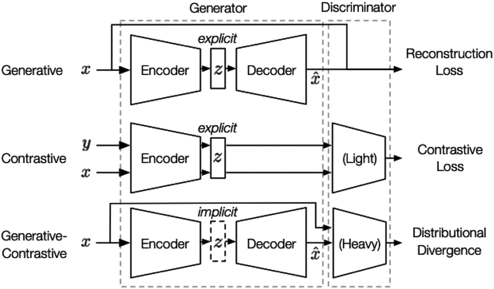
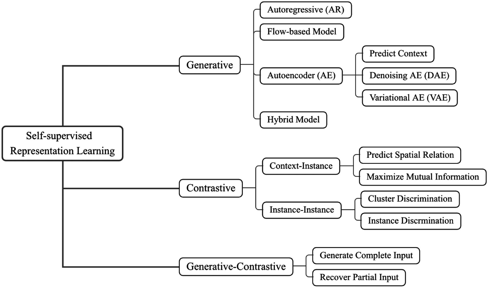
Different authors classify SSL algorithms slightly differently, but based on the pretext tasks, two distinct approaches are identifiable, namely generative and contrastive (see Fig. 2); the other approaches are either a hybrid of these two approaches, namely generative-contrastive / adversarial, or something else entirely.

Fig. 3: Generative, contrastive, as well as a hybrid of generative and contrastive pre-training [LZH+23, Fig. 4]. Generative pre-training does not involve a discriminator. A contrastive discriminator is usually lightweight (e.g., a two/three-layer multilayer perceptron), hence the label “(Light)”.

In Fig. 3, the generative (or generation-based) pre-training pipeline consists of a generator that 1️⃣ uses an encoder to encode input into an explicit vector , and a decoder to reconstruct from as ; 2️⃣ is trained to minimise the reconstruction loss, which is a function of the difference between and .

In Fig. 3, the contrastive (or contrast-based) pre-training pipeline consists of two components:

  1. the generator uses an encoder to encode two versions of the input, namely and which can be related to each other through data augmentation, into two representations;
  2. the discriminator computes the contrastive loss based on the difference between the two representations, so that the generator can be trained to minimise the contrastive loss.

Figs. 4-5 illustrate generative and contrastive pre-training in greater details using graph learning as the context.

Fig. 4: Applying generative SSL to graph learning [LJP+22, Fig. 3(a)]. “Representations” here is equivalent to in Fig. 3.
Fig. 5: Applying contrastive SSL to graph learning [LJP+22, Fig. 3(c)]. The two “Augmented Graphs” here correspond to and in Fig. 3. “Representations” here is equivalent to in Fig. 3. To resolve discrepancies between Fig. 3 and Fig. 5, consider Fig. 5 to be right.

Fig. 5: Classification of self-supervised learning algorithms [LZH+23, Fig. 3].

An extensive list of references on SSL can be found on GitHub.

References

[JT21] L. Jing and Y. Tian, Self-supervised visual feature learning with deep neural networks: A survey, IEEE Transactions on Pattern Analysis and Machine Intelligence 43 no. 11 (2021), 4037–4058. https://doi.org/10.1109/TPAMI.2020.2992393.
[KNH+22] S. Khan, M. Naseer, M. Hayat, S. W. Zamir, F. S. Khan, and M. Shah, Transformers in vision: A survey, ACM Comput. Surv. 54 no. 10s (2022). https://doi.org/10.1145/3505244.
[LJP+22] Y. Liu, M. Jin, S. Pan, C. Zhou, Y. Zheng, F. Xia, and P. Yu, Graph self-supervised learning: A survey, IEEE Transactions on Knowledge and Data Engineering (2022), early access. https://doi.org/10.1109/TKDE.2022.3172903.
[LZH+23] X. Liu, F. Zhang, Z. Hou, L. Mian, Z. Wang, J. Zhang, and J. Tang, Self-supervised learning: Generative or contrastive, IEEE Transactions on Knowledge and Data Engineering 35 no. 1 (2023), 857–876. https://doi.org/10.1109/TKDE.2021.3090866.
[Mur22] K. P. Murphy, Probabilistic Machine Learning: An introduction, MIT Press, 2022. Available at http://probml.ai.

Picture of Yee Wei Law

Standardising/standardisation and whitening

by Yee Wei Law - Tuesday, 20 June 2023, 7:34 AM
 

Given a dataset , where denotes the number of samples and denotes the number of features, it is a common practice to preprocess so that each column has zero mean and unit variance; this is called standardising the data [Mur22, Sec. 7.4.5].

Standardising forces the variance (per column) to be 1 but does not remove correlation between columns.

Decorrelation necessitates whitening.

Whitening is a linear transformation of measurement that produces decorrelated such that the covariance matrix , where is called a whitening matrix [CPSK07, Sec. 2.5.3].

All , and have the same number of rows, denoted ,  which satisfies ; if , then dimensionality reduction is also achieved besides whitening.

A whitening matrix can be obtained using eigenvalue decomposition:

where is an orthogonal matrix containing the covariance matrix’s eigenvectors as its columns, and is the diagonal matrix of the covariance matrix’s eigenvalues [ZX09, p. 74]. Based on the decomposition, the whitening matrix can be defined as

above is called the PCA whitening matrix [Mur22, Sec. 7.4.5].

References

[CPSK07] K. J. Cios, W. Pedrycz, R. W. Swiniarski, and L. A. Kurgan, Data Mining: A Knowledge Discovery Approach, Springer New York, NY, 2007. https://doi.org/10.1007/978-0-387-36795-8.
[Mur22] K. P. Murphy, Probabilistic Machine Learning: An introduction, MIT Press, 2022. Available at http://probml.ai.
[ZX09] N. Zheng and J. Xue, Statistical Learning and Pattern Analysis for Image and Video Processing, Springer London, 2009. https://doi.org/10.1007/978-1-84882-312-9.